import pandas as pd          # 导入数据分析库 pandas
# Import the pandas library for data analysis
import numpy as np           # 导入数值计算库 numpy
# Import the numpy library for numerical computation
import matplotlib.pyplot as plt  # 导入绘图库 matplotlib
# Import the matplotlib library for plotting
import seaborn as sns        # 导入统计可视化库 seaborn
# Import the seaborn library for statistical visualization
import platform              # 导入平台检测库,用于自动适配数据路径
# Import the platform library for OS detection and auto-adapting data paths

# 设置中文字体,确保图表中中文正常显示
# Set Chinese fonts to ensure proper display of Chinese characters in charts
plt.rcParams['font.sans-serif'] = ['SimHei', 'Microsoft YaHei']  # 设置中文字体优先级列表
# Set the priority list of Chinese fonts
# 解决负号显示问题
# Fix the minus sign display issue
plt.rcParams['axes.unicode_minus'] = False  # 修复负号显示为方块的问题
# Fix the issue where minus signs are displayed as squares

# 根据操作系统自动设置本地数据路径
# Automatically set local data paths based on the operating system
if platform.system() == 'Windows':  # 判断当前操作系统类型
# Check the current operating system type
    data_path = 'C:/qiufei/data/stock'  # Windows 数据路径
    # Data path for Windows
else:  # Linux 系统下使用服务器数据路径
# Use server data path on Linux
    data_path = '/home/ubuntu/r2_data_mount/qiufei/data/stock'  # Linux 数据路径
    # Data path for Linux

# 读取上市公司基本信息
# Load basic information of listed companies
stock_basic_dataframe = pd.read_hdf(f'{data_path}/stock_basic_data.h5')  # 加载上市公司基本信息数据
# Load the basic information dataset of listed companies
# 读取前复权日度行情数据
# Load pre-adjusted daily price data
stock_price_dataframe = pd.read_hdf(f'{data_path}/stock_price_pre_adjusted.h5')  # 加载前复权日度股价行情
# Load pre-adjusted daily stock price data
# 重置索引,使 order_book_id 和 date 从索引变为普通列
# Reset the index so that order_book_id and date become regular columns
stock_price_dataframe = stock_price_dataframe.reset_index()  # 将多级索引转为普通列便于筛选操作
# Convert multi-level index to regular columns for easier filtering1 统计学导论 (Introduction to Statistics)
统计学是一门关于数据的科学,它系统地研究数据的收集、整理、分析和解释,从而从数据中提取有价值的信息和知识。在当今这个大数据时代,统计学已经渗透到商业、经济、医学、工程、社会科学等几乎所有领域,成为决策者和研究者不可或缺的工具。对于商学院的学生而言,掌握统计学思维和方法,不仅意味着能够分析数据,更意味着能够在不确定的商业环境中做出理性的、基于证据的决策。
Statistics is the science of data. It systematically studies the collection, organization, analysis, and interpretation of data to extract valuable information and knowledge. In today’s era of big data, statistics has permeated virtually every field—business, economics, medicine, engineering, and the social sciences—making it an indispensable tool for decision-makers and researchers. For business school students, mastering statistical thinking and methods means not only being able to analyze data, but also being able to make rational, evidence-based decisions in an uncertain business environment.
1.0.1 统计学在经济金融领域的典型应用 (Typical Applications of Statistics in Economics and Finance)
统计学是现代金融和经济学研究的基石。对于商学院的学生来说,最重要的不是统计学的历史沿革,而是它今天如何被实际地用于解决真实的商业和金融问题。以下几个典型应用场景,涵盖了本书后续章节将要系统介绍的核心方法,旨在激发学生的学习动力。
Statistics is the cornerstone of modern finance and economics research. For business school students, the most important thing is not the historical evolution of statistics, but rather how it is actually used today to solve real business and financial problems. The following typical application scenarios cover the core methods that will be systematically introduced in subsequent chapters of this book, aiming to inspire students’ motivation to learn.
1.0.1.1 应用一:投资组合风险管理 (Application 1: Portfolio Risk Management)
投资组合管理是金融学的核心议题之一。Harry Markowitz 于 1952 年提出的均值-方差 (Mean-Variance) 框架,其核心思想是:投资者应该在给定的风险水平下最大化预期收益,或在给定的收益水平下最小化风险。这个理论的全部技术工具——均值、方差、协方差、相关系数——正是本书 章节 2 和 章节 8 的核心内容。
Portfolio management is one of the core topics in finance. The Mean-Variance framework proposed by Harry Markowitz in 1952 is based on the idea that investors should maximize expected return for a given level of risk, or minimize risk for a given level of return. All the technical tools of this theory—mean, variance, covariance, and correlation coefficient—are precisely the core content of 章节 2 and 章节 8 in this book.
一位量化基金经理的日常工作流程大致如下:
The daily workflow of a quantitative fund manager roughly involves the following:
计算收益率的描述统计量(第二章): 均值代表预期收益,标准差代表风险
构建相关系数矩阵(第八章): 理解资产之间的联动关系,这是分散化投资的关键
进行回归分析(第八章、第十章): 估计资产的 Beta 系数,量化系统性风险敞口
假设检验(第五章、第七章): 评估投资策略的 Alpha 是否统计显著,即超额收益是能力还是运气
Computing descriptive statistics of returns (Chapter 2): The mean represents expected return; the standard deviation represents risk
Constructing a correlation matrix (Chapter 8): Understanding the co-movement between assets, which is key to diversification
Performing regression analysis (Chapters 8 and 10): Estimating the Beta coefficient of assets to quantify systematic risk exposure
Hypothesis testing (Chapters 5 and 7): Evaluating whether the Alpha of an investment strategy is statistically significant—i.e., whether excess returns are due to skill or luck
我们来用中国A股市场的真实数据,快速预览一下统计学在投资分析中的应用:
Let us use real data from China’s A-share market to quickly preview the application of statistics in investment analysis:
本地股票基本信息和行情数据加载完毕。下面选取5家长三角代表性上市公司2023年数据,并计算日对数收益率。
Local stock basic information and price data have been loaded. Next, we select 5 representative listed companies from the Yangtze River Delta region for 2023 data and calculate daily log returns.
# 选取5家长三角代表性上市公司
# Select 5 representative listed companies from the Yangtze River Delta
# 海康威视(杭州)、宁波银行(宁波)、恒瑞医药(连云港)、科大讯飞(合肥)、上汽集团(上海)
# Hikvision (Hangzhou), Bank of Ningbo (Ningbo), Hengrui Medicine (Lianyungang), iFlytek (Hefei), SAIC Motor (Shanghai)
selected_stock_id_list = [  # 初始化长三角代表性公司股票代码列表
# Initialize the stock code list of representative YRD companies
    '002415.XSHE',  # 海康威视 - 安防科技龙头
    # Hikvision - Leading security technology company
    '002142.XSHE',  # 宁波银行 - 城商行标杆
    # Bank of Ningbo - Benchmark city commercial bank
    '600276.XSHG',  # 恒瑞医药 - 创新药龙头
    # Hengrui Medicine - Leading innovative pharmaceutical company
    '002230.XSHE',  # 科大讯飞 - AI语音龙头
    # iFlytek - Leading AI voice technology company
    '600104.XSHG',  # 上汽集团 - 汽车制造龙头
    # SAIC Motor - Leading automobile manufacturer
]  # 完成长三角地区5家代表性上市公司的股票代码列表定义
# Completed the definition of the stock code list for 5 representative YRD companies

# 筛选这5家公司2023年全年的行情数据,并复制以避免 SettingWithCopyWarning
# Filter the 2023 full-year price data for these 5 companies, copying to avoid SettingWithCopyWarning
filtered_price_2023 = stock_price_dataframe[  # 基于布尔索引筛选目标股票和日期范围
# Filter target stocks and date range using boolean indexing
    (stock_price_dataframe['order_book_id'].isin(selected_stock_id_list)) &  # 股票代码在选定列表中
    # Stock code is in the selected list
    (stock_price_dataframe['date'] >= '2023-01-01') &  # 日期不早于2023年1月1日
    # Date is no earlier than January 1, 2023
    (stock_price_dataframe['date'] <= '2023-12-31')  # 日期不晚于2023年12月31日
    # Date is no later than December 31, 2023
].copy()  # 复制数据避免 SettingWithCopyWarning
# Copy data to avoid SettingWithCopyWarning

# 将数据从长格式 (long format) 转换为宽格式 (wide format)
# Convert data from long format to wide format
# 每一列代表一只股票的收盘价,每一行代表一个交易日
# Each column represents a stock's closing price; each row represents a trading day
pivoted_close_price = filtered_price_2023.pivot(  # 将长格式数据透视为宽格式(每列一只股票)
# Pivot long-format data into wide format (one stock per column)
    index='date',            # 以日期为行索引
    # Use date as the row index
    columns='order_book_id', # 以股票代码为列名
    # Use stock code as column names
    values='close'           # 提取收盘价
    # Extract closing prices
)  # 完成数据透视,得到以日期为行、股票为列的收盘价宽格式矩阵
# Completed the pivot, obtaining a wide-format matrix of closing prices with dates as rows and stocks as columns

# 计算日对数收益率: ln(P_t / P_{t-1})
# Calculate daily log returns: ln(P_t / P_{t-1})
# 对数收益率具有时间可加性,是金融学中的标准做法
# Log returns have the property of time additivity, which is standard practice in finance
daily_log_returns = np.log(pivoted_close_price / pivoted_close_price.shift(1)).dropna()  # 计算日对数收益率并删除首行缺失值
# Calculate daily log returns and drop the first row with missing values
上述代码完成了数据加载、筛选和对数收益率计算。下面将列名替换为公司简称,并绘制相关性热力图。
The above code completes data loading, filtering, and log return calculation. Next, we replace column names with company abbreviations and plot the correlation heatmap.
# 将列名从股票代码替换为更易读的公司简称
# Replace column names from stock codes to more readable company abbreviations
stock_name_mapping = {  # 构建股票代码到公司简称的映射字典
# Build a mapping dictionary from stock codes to company abbreviations
    '002415.XSHE': '海康威视',  # 杭州,安防科技龙头
    # Hangzhou, leading security technology company
    '002142.XSHE': '宁波银行',  # 宁波,城商行标杆
    # Ningbo, benchmark city commercial bank
    '600276.XSHG': '恒瑞医药',  # 连云港,创新药龙头
    # Lianyungang, leading innovative pharmaceutical company
    '002230.XSHE': '科大讯飞',  # 合肥,AI语音龙头
    # Hefei, leading AI voice technology company
    '600104.XSHG': '上汽集团',  # 上海,汽车制造龙头
    # Shanghai, leading automobile manufacturer
}  # 完成股票代码到公司简称的映射字典定义
# Completed the definition of the mapping dictionary from stock codes to company abbreviations
daily_log_returns.columns = [stock_name_mapping[col] for col in daily_log_returns.columns]  # 将列名从股票代码替换为公司简称
# Replace column names from stock codes to company abbreviations

# 计算相关系数矩阵: 衡量任意两只股票收益率的线性关联程度
# Calculate the correlation matrix: measure the degree of linear association between any two stocks' returns
correlation_matrix = daily_log_returns.corr()  # 计算Pearson相关系数矩阵
# Compute the Pearson correlation coefficient matrix

# 绘制热力图: 直观展示资产间的相关性结构
# Plot a heatmap: visually display the correlation structure among assets
fig, axis = plt.subplots(figsize=(8, 6))  # 创建8x6英寸的画布
# Create an 8x6-inch canvas
sns.heatmap(  # 绘制相关系数热力图
# Plot the correlation coefficient heatmap
    correlation_matrix,      # 传入相关系数矩阵
    # Pass in the correlation matrix
    annot=True,              # 在每个格子中显示数值
    # Display values in each cell
    fmt='.2f',               # 保留两位小数
    # Keep two decimal places
    cmap='RdBu_r',           # 使用红蓝配色方案(红色=正相关,蓝色=负相关)
    # Use the red-blue color scheme (red = positive correlation, blue = negative correlation)
    center=0,                # 将颜色中心设为0
    # Set the color center to 0
    vmin=-1, vmax=1,         # 相关系数的取值范围为[-1, 1]
    # The range of correlation coefficients is [-1, 1]
    square=True,             # 让每个格子为正方形
    # Make each cell square
    ax=axis                  # 指定绑图坐标轴
    # Specify the plotting axis
)  # 完成相关性热力图的绑制参数配置
# Completed the configuration of heatmap plotting parameters
axis.set_title('长三角上市公司日收益率相关性(2023年)', fontsize=14)  # 设置热力图标题
# Set the heatmap title
plt.tight_layout()           # 自动调整布局,防止标签被截断
# Automatically adjust layout to prevent label clipping
plt.show()  # 渲染并展示图形
# Render and display the figure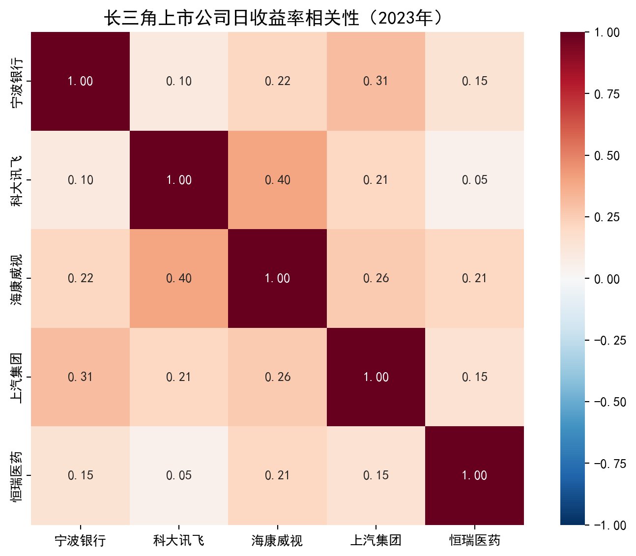
上图展示的相关系数矩阵揭示了一个重要信息:不同行业的股票之间相关性较低,这意味着将它们组合在一起可以有效分散风险——这正是 Markowitz 投资组合理论的核心洞察。我们将在 章节 8 中系统学习相关系数的计算与检验方法。
The correlation matrix shown above reveals an important insight: stocks from different industries have relatively low correlations, meaning that combining them can effectively diversify risk—this is precisely the core insight of Markowitz’s portfolio theory. We will systematically study the calculation and testing of correlation coefficients in 章节 8.
1.0.1.2 应用二:上市公司财务质量的统计评估 (Application 2: Statistical Assessment of Listed Company Financial Quality)
在基本面分析中,投资者需要从数以千计的上市公司中筛选出财务质量优良的标的。这一过程大量使用描述统计( 章节 2 )和推断统计( 章节 5 )的方法:
In fundamental analysis, investors need to screen thousands of listed companies to identify those with excellent financial quality. This process extensively uses methods of descriptive statistics ( 章节 2 ) and inferential statistics ( 章节 5 ):
描述统计:计算全市场公司的营收增长率、净资产收益率 (ROE)、资产负债率等指标的均值、中位数、标准差,从而建立”行业基准” (benchmark)
概率分布:财务指标的分布形态(是否正态、是否存在偏态和厚尾)直接影响我们选择哪种统计方法进行分析( 章节 4 )
假设检验:例如,检验长三角地区上市公司的 ROE 是否显著高于全国平均水平( 章节 7 )
回归分析:探究影响公司盈利能力的关键因素,如研发投入、资产规模、财务杠杆等( 章节 10 )
Descriptive statistics: Calculate the mean, median, and standard deviation of metrics such as revenue growth rate, return on equity (ROE), and debt-to-asset ratio for all listed companies, thereby establishing “industry benchmarks”
Probability distributions: The distributional shape of financial indicators (whether normal, skewed, or heavy-tailed) directly affects which statistical methods we choose for analysis ( 章节 4 )
Hypothesis testing: For example, testing whether the ROE of companies in the Yangtze River Delta region is significantly higher than the national average ( 章节 7 )
Regression analysis: Investigating key factors affecting corporate profitability, such as R&D investment, asset size, and financial leverage ( 章节 10 )
1.0.1.3 应用三:量化因子投资 (Application 3: Quantitative Factor Investing)
在中国资本市场,量化投资已经成为一种主流的投资策略。其核心思想是:构建一系列能够预测股票未来收益的”因子”(factor),如市盈率 (PE)、市净率 (PB)、市值 (Market Cap)、动量 (Momentum) 等,然后通过多元回归模型( 章节 10 )和机器学习方法( 章节 12 、 章节 13 )来构建选股模型。
In the Chinese capital market, quantitative investing has become a mainstream investment strategy. Its core idea is to construct a set of “factors” that can predict future stock returns—such as price-to-earnings ratio (PE), price-to-book ratio (PB), market capitalization, and momentum—and then use multiple regression models ( 章节 10 ) and machine learning methods ( 章节 12, 章节 13 ) to build stock selection models.
一个完整的因子投资研究流程涉及本书几乎所有的统计方法:
A complete factor investing research process involves almost all the statistical methods in this book:
探索性数据分析( 章节 2 ):理解因子的分布特征和截面差异
相关性分析( 章节 8 ):检验因子之间的多重共线性
回归分析( 章节 10 ):估计因子对收益率的边际贡献
方差分析( 章节 9 ):比较不同因子组合的策略表现是否有显著差异
非线性模型( 章节 11 ):当因子与收益率之间的关系不是简单线性时,需要使用逻辑回归等非线性方法
树模型和集成学习( 章节 12 ):处理高维因子的非线性交互效应
聚类分析( 章节 13 ):将股票根据因子特征进行无监督分类,发现市场的内在结构
Exploratory data analysis ( 章节 2 ): Understanding the distributional characteristics and cross-sectional differences of factors
Correlation analysis ( 章节 8 ): Testing multicollinearity among factors
Regression analysis ( 章节 10 ): Estimating the marginal contribution of each factor to returns
Analysis of variance ( 章节 9 ): Comparing whether the performance of different factor combinations differs significantly
Nonlinear models ( 章节 11 ): When the relationship between factors and returns is not simply linear, nonlinear methods such as logistic regression are needed
Tree models and ensemble learning ( 章节 12 ): Handling nonlinear interaction effects of high-dimensional factors
Cluster analysis ( 章节 13 ): Unsupervised classification of stocks based on factor characteristics to discover the intrinsic structure of the market
1.0.1.4 应用四:宏观经济与货币政策分析 (Application 4: Macroeconomic and Monetary Policy Analysis)
宏观经济数据(GDP增长率、CPI、PMI、M2增速等)是影响资本市场走势的关键因素。经济学家和分析师大量使用时间序列分析方法来研究宏观经济变量之间的动态关系。虽然本书侧重于截面数据和面板数据的方法,但其中许多核心概念——如回归分析、自变量选择、模型诊断——在时间序列分析中同样适用。
Macroeconomic data (GDP growth rate, CPI, PMI, M2 growth rate, etc.) are key factors influencing the trends of capital markets. Economists and analysts extensively use time series analysis methods to study the dynamic relationships among macroeconomic variables. Although this book focuses on cross-sectional and panel data methods, many of its core concepts—such as regression analysis, variable selection, and model diagnostics—are equally applicable in time series analysis.
例如,中国央行在制定货币政策时,会使用统计模型来评估利率调整对经济增长和物价稳定的影响。投资者也会利用回归模型来分析宏观经济指标对股票市场的传导机制。
For example, when formulating monetary policy, the People’s Bank of China uses statistical models to assess the impact of interest rate adjustments on economic growth and price stability. Investors also use regression models to analyze the transmission mechanism of macroeconomic indicators to the stock market.
小结:统计学是金融决策的语言
Summary: Statistics is the Language of Financial Decision-Making
从以上四个应用场景可以看出,统计学不是一门抽象的数学理论,而是金融从业者每天都在使用的实用工具。无论是投资组合管理、公司财务分析、量化策略开发,还是宏观经济研究,统计方法无处不在。本书的目标,就是帮助商学院的学生系统地掌握这些方法,并能够将其应用于中国资本市场的真实数据分析之中。
From the above four application scenarios, we can see that statistics is not an abstract mathematical theory, but a practical tool used daily by finance professionals. Whether it is portfolio management, corporate financial analysis, quantitative strategy development, or macroeconomic research, statistical methods are ubiquitous. The goal of this book is to help business school students systematically master these methods and apply them to real data analysis in China’s capital markets.
1.1 统计学在商业决策中的核心作用 (The Core Role of Statistics in Business Decision-Making)
1.1.1 案例研究:A/B测试在券商量化策略中的应用 (Case Study: A/B Testing in Securities Firm Quantitative Strategies)
让我们通过一个中国证券行业的真实案例来理解统计学的核心价值。
Let us understand the core value of statistics through a real case from China’s securities industry.
1.1.1.1 背景:券商量化选股策略优化 (Background: Optimization of Securities Firm Quantitative Stock Selection Strategy)
某头部券商的量化投研团队管理着超过200亿元的资产。为了提升组合的超额收益(Alpha),团队开发了一种新的多因子选股模型,声称可以提高策略的月度胜率(Win Rate)。
A leading securities firm’s quantitative investment research team manages over 20 billion yuan in assets. To improve the portfolio’s excess return (Alpha), the team developed a new multi-factor stock selection model, claiming it could improve the strategy’s monthly win rate.
1.1.1.2 实验设计 (Experimental Design)
为了验证这个新模型是否真的有效,他们设计了如下随机对照实验:
To verify whether this new model is truly effective, they designed the following randomized controlled experiment:
实验参数:
Experimental Parameters:
实验周期:12个月回测
样本规模:20,000次模拟交易信号
随机分配:10,000次信号使用新模型,10,000次使用旧模型
Experimental period: 12-month backtest
Sample size: 20,000 simulated trading signals
Random assignment: 10,000 signals use the new model, 10,000 use the old model
分组方案:
Group Assignment:
处理组(Treatment Group):使用新多因子选股模型
对照组(Control Group):使用原选股模型
Treatment Group: Uses the new multi-factor stock selection model
Control Group: Uses the original stock selection model
1.1.1.3 实验结果 (Experimental Results)
如 表 1.1 所示,实验结果显示处理组的月度胜率(25%)比对照组(22%)高出3个百分点。
As shown in 表 1.1, the experimental results show that the treatment group’s monthly win rate (25%) is 3 percentage points higher than the control group (22%).
# ========== 导入所需库 ==========
# ========== Import required libraries ==========
import pandas as pd  # 导入数据分析库 pandas
# Import the pandas data analysis library

# ========== 构建A/B测试结果数据 ==========
# ========== Build A/B test result data ==========
# 演示用模拟数据 (Mock data for demonstration)
# Mock data for demonstration
# 场景:某头部券商量化团队对比新旧选股模型的效果
# Scenario: A leading securities firm's quant team compares new vs. old stock selection models
ab_test_data_dict = {  # 构建A/B测试结果的数据字典
# Build the data dictionary for A/B test results
    '组别': ['处理组(新因子模型)', '对照组(旧因子模型)'],  # 实验分组名称
    # Experimental group names
    '模拟交易信号数': [10000, 10000],  # 每组产生的模拟交易信号数量
    # Number of simulated trading signals per group
    '月度胜出信号数': [2500, 2200],  # 信号产生正收益的次数
    # Number of signals that generated positive returns
    '月度胜率': ['25%', '22%']  # 胜出信号数 / 总信号数
    # Win rate = winning signals / total signals
}  # 完成A/B测试结果数据字典的构建
# Completed the construction of the A/B test result data dictionary

# ========== 创建并展示结果表格 ==========
# ========== Create and display the results table ==========
ab_test_results_dataframe = pd.DataFrame(ab_test_data_dict)  # 将字典转为 DataFrame
# Convert the dictionary to a DataFrame
ab_test_results_dataframe  # 输出表格
# Output the table| 组别 | 模拟交易信号数 | 月度胜出信号数 | 月度胜率 | |
|---|---|---|---|---|
| 0 | 处理组(新因子模型) | 10000 | 2500 | 25% |
| 1 | 对照组(旧因子模型) | 10000 | 2200 | 22% |
1.1.1.4 统计学的核心问题 (The Core Question of Statistics)
这3个百分点的差异是真实的、由新因子模型带来的效果,还是仅仅由于随机波动造成的偶然结果?
Is this 3-percentage-point difference a real effect brought by the new factor model, or merely a chance result caused by random fluctuation?
这就是统计学的核心问题。现实世界中,数据总是包含着自然变异(natural variation)。即使新旧模型完全相同,处理组和对照组的月度胜率也会因为随机性而略有差异。
This is the core question of statistics. In the real world, data always contains natural variation. Even if the new and old models were exactly the same, the monthly win rates of the treatment and control groups would still differ slightly due to randomness.
直觉可视化:大数定律 (Law of Large Numbers)
Intuitive Visualization: The Law of Large Numbers
为什么我们相信样本能代表总体?核心基石是大数定律。 它告诉我们:随着样本量 \(n\) 的增加,样本均值 \(\bar{X}\) 会以概率 1 收敛到总体均值 \(\mu\)。
Why do we believe that a sample can represent a population? The cornerstone is the Law of Large Numbers. It tells us that as the sample size \(n\) increases, the sample mean \(\bar{X}\) converges to the population mean \(\mu\) with probability 1.
我们可以通过一个简单的 Python 模拟来”看见”这个定律。
We can “see” this law through a simple Python simulation.
# ========== 导入所需库 ==========
# ========== Import required libraries ==========
import numpy as np           # 导入数值计算库
# Import the numerical computation library
import matplotlib.pyplot as plt  # 导入绑图库
# Import the plotting library

# ========== 模拟抛硬币实验 ==========
# ========== Simulate coin-flipping experiment ==========
np.random.seed(42)  # 设定随机数种子,确保结果可复现
# Set random seed for reproducibility
num_coin_flip_trials = 2000  # 总抛掷次数设为2000次
# Set total number of flips to 2000
coin_flip_results = np.random.randint(0, 2, num_coin_flip_trials)  # 生成2000个0或1的随机数(0=反面, 1=正面)
# Generate 2000 random integers of 0 or 1 (0 = tails, 1 = heads)
# 计算累积正面频率: 前 n 次中正面出现的比例
# Calculate cumulative heads frequency: proportion of heads in the first n flips
cumulative_mean_frequencies = np.cumsum(coin_flip_results) / (np.arange(num_coin_flip_trials) + 1)  # 计算前n次抛掷中正面出现的累积频率
# Calculate the cumulative frequency of heads in the first n flips

# ========== 绘制大数定律可视化图 ==========
# ========== Plot the Law of Large Numbers visualization ==========
plt.figure(figsize=(10, 5))  # 创建10x5英寸的画布
# Create a 10x5-inch canvas
plt.plot(cumulative_mean_frequencies, color='#2C3E50', linewidth=1.5, label='累积正面频率')  # 绘制频率曲线
# Plot the frequency curve
plt.axhline(0.5, color='#E3120B', linestyle='--', linewidth=2, label='理论概率 (0.5)')  # 绘制理论值参考线
# Plot the theoretical value reference line
plt.xlabel('抛掷次数', fontsize=12)  # X轴标签
# X-axis label
plt.ylabel('正面出现的频率', fontsize=12)  # Y轴标签
# Y-axis label
plt.title('大数定律可视化: 频率收敛于概率', fontsize=14)  # 图标题
# Chart title
plt.legend()  # 显示图例
# Display legend
plt.grid(True, alpha=0.3)  # 显示网格线,透明度为0.3
# Display grid lines with 0.3 transparency
plt.show()  # 展示图形
# Display the figure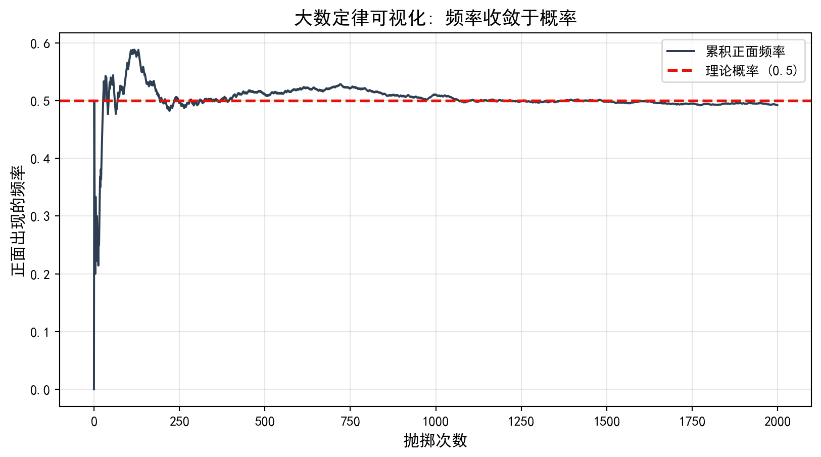
注意看图的前半部分:当次数很少时,频率波动巨大(可能连续几次正面,频率100%)。但随着次数增加,这条线就像被一种引力吸住一样,稳定在 0.5 附近。这就是统计推断的信心来源——数据越多,真相越清晰。
Pay attention to the first half of the chart: when the number of flips is small, the frequency fluctuates wildly (there might be several consecutive heads, bringing the frequency to 100%). But as the number of flips increases, the line is pulled as if by gravity, stabilizing around 0.5. This is the source of confidence in statistical inference—the more data, the clearer the truth.
1.2 数据基础与变量类型 (Data Fundamentals and Variable Types)
1.2.1 数据框结构 (Data Frame Structure)
在Python中,pandas库提供的DataFrame是处理统计数据的核心数据结构。数据框(data frame)是一个二维表格,其中:
In Python, the DataFrame provided by the pandas library is the core data structure for handling statistical data. A data frame is a two-dimensional table in which:
每一行(row):代表一个观测单元(observation)或案例(case)
每一列(column):代表一个变量(variable)
Each row: represents an observation unit or case
Each column: represents a variable
让我们通过一个真实的A股市场数据示例来理解数据框结构。如 表 1.2 所示,我们展示了2023年中国长三角地区部分上市公司的基本信息。
Let us understand the data frame structure through a real example from the A-share market. As shown in 表 1.2, we display the basic information of some listed companies in China’s Yangtze River Delta region.
# ========== 导入所需库 ==========
# ========== Import required libraries ==========
import pandas as pd   # 导入数据分析库 pandas
# Import the pandas data analysis library
import platform       # 导入平台检测库,用于自动适配数据路径
# Import the platform detection library for auto-adapting data paths

# ========== 设置本地数据路径 ==========
# ========== Set local data paths ==========
if platform.system() == 'Windows':  # 判断当前操作系统类型
# Check the current operating system type
    data_path = 'C:/qiufei/data/stock'  # Windows 数据路径
    # Data path for Windows
else:  # Linux 系统下使用服务器数据路径
# Use server data path on Linux
    data_path = '/home/ubuntu/r2_data_mount/qiufei/data/stock'  # Linux 数据路径
    # Data path for Linux

# ========== 读取并筛选数据 ==========
# ========== Load and filter data ==========
stock_basic_dataframe = pd.read_hdf(f'{data_path}/stock_basic_data.h5')  # 读取上市公司基本信息
# Load basic information of listed companies

# 定义长三角地区包含的省份列表
# Define the list of provinces in the Yangtze River Delta region
yangtze_delta_city_list = ['上海市', '浙江省', '江苏省', '安徽省']  # 长三角四省市对应的行政区划名称
# Administrative division names for the four YRD provinces/municipalities
# 筛选注册地在长三角地区的公司,取前10条做示例展示
# Filter companies registered in the YRD region, take the first 10 for demonstration
sampled_stock_dataframe = stock_basic_dataframe[stock_basic_dataframe['province'].isin(yangtze_delta_city_list)].head(10)  # 筛选长三角公司并取前10条
# Filter YRD companies and take the first 10

# ========== 输出结果 ==========
# ========== Output results ==========
print(f'数据框维度: {sampled_stock_dataframe.shape[0]}行 {sampled_stock_dataframe.shape[1]}列')  # 打印数据框的行数和列数
# Print the number of rows and columns of the data frame
# 选取关键字段展示: 股票代码、简称、省份、行业、上市日期
# Select key fields for display: stock code, abbreviation, province, industry, listing date
sampled_stock_dataframe[['order_book_id', 'abbrev_symbol', 'province', 'industry_name', 'listed_date']]  # 输出选定字段的数据表
# Output the data table with selected fields
数据框维度: 10行 24列| order_book_id | abbrev_symbol | province | industry_name | listed_date | |
|---|---|---|---|---|---|
| 34 | 000035.XSHE | ZGTY | 江苏省 | 生态保护和环境治理业 | 1994-04-08 |
| 70 | 000153.XSHE | FYYY | 安徽省 | 医药制造业 | 2000-09-20 |
| 72 | 000156.XSHE | HSCM | 浙江省 | 广播、电视、电影和影视录音制作业 | 2000-09-06 |
| 77 | 000301.XSHE | DFSH | 江苏省 | 化学纤维制造业 | 2000-05-29 |
| 91 | 000411.XSHE | YTJT | 浙江省 | 批发业 | 1996-07-16 |
| 96 | 000417.XSHE | HBJT | 安徽省 | 零售业 | 1996-08-12 |
| 97 | 000418.XSHE | XTEA | 江苏省 | 未知 | 1997-03-28 |
| 100 | 000421.XSHE | NJGY | 江苏省 | 燃气生产和供应业 | 1996-08-06 |
| 103 | 000425.XSHE | XGJX | 江苏省 | 专用设备制造业 | 1996-08-28 |
| 125 | 000517.XSHE | RADC | 浙江省 | 房地产业 | 1993-08-06 |
上面的代码从本地数据文件中读取了中国A股上市公司的基本信息,并筛选出长三角地区(上海、浙江、江苏、安徽)的公司样本。表 1.2 的输出结果是一个典型的数据框:表中每一行对应一家上市公司(即一个观测单元),各列则代表不同的变量,如 order_book_id(股票代码)、abbrev_symbol(股票简称)、province(注册省份)、industry_name(所属行业)和 listed_date(上市日期)。这种”行=观测、列=变量”的二维表格结构,就是贯穿整本教材的核心数据组织形式。
The above code reads the basic information of Chinese A-share listed companies from local data files, filtering for companies in the Yangtze River Delta region (Shanghai, Zhejiang, Jiangsu, and Anhui). The output of 表 1.2 is a typical data frame: each row corresponds to a listed company (i.e., an observation unit), and each column represents a different variable, such as order_book_id (stock code), abbrev_symbol (stock abbreviation), province (registered province), industry_name (industry classification), and listed_date (listing date). This “row = observation, column = variable” two-dimensional table structure is the core data organization form used throughout this textbook.
1.2.2 变量的类型体系 (The Variable Type System)
理解变量类型是统计分析的基础。如 图 1.3 所示,变量可以分为两大类:数值变量和分类变量。
Understanding variable types is the foundation of statistical analysis. As shown in 图 1.3, variables can be divided into two broad categories: numerical variables and categorical variables.
1.2.2.1 1. 数值变量 (Numerical/Quantitative Variables)
数值变量可以取具体的数值,可以进行算术运算。
Numerical variables take specific numeric values and can be subjected to arithmetic operations.
离散变量(Discrete Variables):只能取离散的、分离的值,通常是整数计数。
Discrete Variables: Can only take discrete, separated values, usually integer counts.
- 特征:可能取值是可数的(0, 1, 2, 3…)
- 中国商业案例:
- 阿里巴巴的年度活跃用户数:10.39亿(2024财年)
- 上汽集团的年销量:约500万辆
- 每日A股成交订单数:数千万笔
- Characteristics: Possible values are countable (0, 1, 2, 3…)
- Chinese business examples:
- Alibaba’s annual active users: 1.039 billion (FY2024)
- SAIC Motor’s annual sales: approximately 5 million vehicles
- Daily A-share trading orders: tens of millions
连续变量(Continuous Variables):可以在一个范围内取任何值,理论上可以无限细分。
Continuous Variables: Can take any value within a range, theoretically infinitely divisible.
- 特征:可能取值是无限可分的
- 中国商业案例:
- 海康威视股价:30-40元/股(可精确到0.01元)
- 海康威视年营收:891.6亿元(2023年)
- 上汽集团汽车产量:502万辆(可精确到辆)
- Characteristics: Possible values are infinitely divisible
- Chinese business examples:
- Hikvision stock price: 30–40 yuan/share (precise to 0.01 yuan)
- Hikvision annual revenue: 89.16 billion yuan (2023)
- SAIC Motor vehicle production: 5.02 million units (precise to the individual unit)
离散 vs 连续的判断准则 (Criteria for Distinguishing Discrete vs. Continuous)
判断一个变量是离散还是连续,关键看可能取值之间是否有”间隙”:
The key to determining whether a variable is discrete or continuous is whether there are “gaps” between possible values:
问题:公司的年收入是离散还是连续?
Question: Is a company’s annual revenue discrete or continuous?
分析:
Analysis:
理论上,收入可以取任何正值,是连续的
但实践中,我们记录到万元或亿元单位
判断标准:这个变量能否取更精细的值?如果能,则是连续的
In theory, revenue can take any positive value and is continuous
In practice, we record it in units of ten thousand or hundred million yuan
Criterion: Can this variable take more precise values? If yes, it is continuous
结论:年收入是连续变量,因为理论上可以精确到分。
Conclusion: Annual revenue is a continuous variable because, in theory, it can be precise to the cent.
1.2.2.2 2. 分类变量 (Categorical/Qualitative Variables)
分类变量代表类别或标签,不能进行算术运算。
Categorical variables represent categories or labels and cannot be subjected to arithmetic operations.
名义变量(Nominal Variables):代表类别或标签,没有内在顺序。
Nominal Variables: Represent categories or labels with no inherent order.
- 特征:类别之间没有优先级或顺序
- 中国商业案例:
- 证券交易所:上交所(SH) vs 深交所(SZ) vs 北交所(BJ)
- 行业分类:金融、科技、制造、消费、医药
- 支付方式:微信支付、支付宝、银联卡、现金
- 公司总部所在地:上海、北京、深圳、杭州
- Characteristics: No priority or ordering among categories
- Chinese business examples:
- Stock exchanges: SSE (SH) vs. SZSE (SZ) vs. BSE (BJ)
- Industry classification: Finance, Technology, Manufacturing, Consumer, Pharmaceuticals
- Payment methods: WeChat Pay, Alipay, UnionPay card, Cash
- Company headquarters: Shanghai, Beijing, Shenzhen, Hangzhou
名义变量的不同取值称为水平(levels)或类别。
The different values of a nominal variable are called levels or categories.
有序变量(Ordinal Variables):具有顺序或排名,但水平之间的间隔不一定均匀。
Ordinal Variables: Have order or ranking, but the intervals between levels are not necessarily uniform.
- 特征:有顺序关系,但间隔不确定
- 中国商业案例:
- 信用评级:AAA > AA > A > BBB(相邻级别之间的风险差异不等)
- 股票分析师评级:强烈买入 > 买入 > 持有 > 卖出 > 强烈卖出
- 客户满意度:非常满意 > 满意 > 一般 > 不满意 > 非常不满意
- 教育程度:博士 > 硕士 > 本科 > 大专 > 高中
- Characteristics: Have ordering relationships, but intervals are uncertain
- Chinese business examples:
- Credit ratings: AAA > AA > A > BBB (risk differences between adjacent levels are not equal)
- Stock analyst ratings: Strong Buy > Buy > Hold > Sell > Strong Sell
- Customer satisfaction: Very Satisfied > Satisfied > Neutral > Dissatisfied > Very Dissatisfied
- Education level: Doctorate > Master’s > Bachelor’s > Associate > High School
重要警示:数字不等于数值变量 (Important Warning: Numbers Do Not Equal Numerical Variables)
这是一个常见的陷阱!有些变量用数字表示但其实是分类变量。
This is a common trap! Some variables are represented by numbers but are actually categorical variables.
典型案例:
Typical examples:
- 邮政编码:上海200000,北京100000
- 计算”平均邮政编码”没有意义
- 这是名义变量
- Postal codes: Shanghai 200000, Beijing 100000
- Calculating an “average postal code” is meaningless
- This is a nominal variable
- 身份证号:虽然全是数字,但完全不能进行算术运算
- 这是名义变量
- National ID numbers: Although entirely composed of digits, arithmetic operations are completely meaningless
- This is a nominal variable
- 股票代码:600000(浦发银行),002142(宁波银行)
- 只是标识符,不能加减乘除
- 这是名义变量
- Stock codes: 600000 (SPD Bank), 002142 (Bank of Ningbo)
- These are merely identifiers; arithmetic operations are meaningless
- This is a nominal variable
- Likert量表:1=非常不同意,2=不同意,3=中立,4=同意,5=非常同意
- 可以计算均值(有争议),但要注意间隔不一定相等
- 通常作为有序变量处理
- Likert scale: 1 = Strongly Disagree, 2 = Disagree, 3 = Neutral, 4 = Agree, 5 = Strongly Agree
- One can compute the mean (controversial), but note that intervals are not necessarily equal
- Usually treated as an ordinal variable
判断标准:对这个变量进行算术运算(加、减、乘、除)是否有实际意义?
Criterion: Do arithmetic operations (addition, subtraction, multiplication, division) on this variable have practical meaning?
1.2.3 变量类型与统计方法的关系 (The Relationship Between Variable Types and Statistical Methods)
不同的变量类型适合不同的统计方法,这在后续章节会详细讨论。
Different variable types are suitable for different statistical methods, which will be discussed in detail in subsequent chapters.
对于数值变量(无论是离散还是连续):
For numerical variables (whether discrete or continuous):
可以计算:均值、中位数、方差、标准差
可以进行:加减乘除、对数变换、标准化
适合使用:t检验、方差分析、回归分析、相关分析
Can compute: mean, median, variance, standard deviation
Can perform: arithmetic, logarithmic transformation, standardization
Suitable methods: t-test, ANOVA, regression analysis, correlation analysis
对于分类变量(无论是名义还是有序):
For categorical variables (whether nominal or ordinal):
只能计算:频数、频率、百分比
适合使用:卡方检验、列联表分析、逻辑回归
Can only compute: frequency, relative frequency, percentage
Suitable methods: chi-square test, contingency table analysis, logistic regression
实践中的处理方式 (Practical Handling)
在实际数据分析中,有时会将分类变量转换为数值变量:
In practice, categorical variables are sometimes converted to numerical variables:
示例:将性别(男/女)转换为虚拟变量(0/1)
Example: Converting gender (male/female) to a dummy variable (0/1)
男 = 0, 女 = 1
这样就可以在回归分析中使用
但要注意:0和1只是编码,不是真正的数值
Male = 0, Female = 1
This allows use in regression analysis
But note: 0 and 1 are just codes, not real numerical values
示例:将教育程度转换为数值
Example: Converting education level to numerical values
高中=12,本科=16,硕士=18,博士=21
使用受教育年限代表教育程度
这样就变成了数值变量
High school = 12, Bachelor’s = 16, Master’s = 18, Doctorate = 21
Using years of education to represent education level
This transforms it into a numerical variable
1.3 变量之间的关系 (Relationships Between Variables)
在实际商业分析中,我们不仅关注单个变量,更关注变量之间的关系。以下通过三个中国金融市场案例来展示不同类型的变量关系。
In real business analysis, we are interested not only in individual variables but also in the relationships between variables. The following three cases from the Chinese financial market illustrate different types of variable relationships.
1.3.0.1 案例1:负相关关系 - 海康威视股价与成交量 (Case 1: Negative Association — Hikvision Stock Price vs. Trading Volume)
公司股价与成交量之间存在着怎样的关系?这是投资分析中的经典议题。我们将以海康威视(002415.XSHE)——中国安防行业龙头、长三角代表性上市公司——为研究对象,利用其2023年全年的真实交易数据进行分析。
What is the relationship between a company’s stock price and its trading volume? This is a classic topic in investment analysis. We will study Hikvision (002415.XSHE) — the leading company in China’s security industry and a representative listed company in the Yangtze River Delta — using its real trading data for the entire year of 2023.
# ========== 导入所需库 ==========
# ========== Import required libraries ==========
import pandas as pd          # 数据分析库
# Data analysis library
import numpy as np           # 数值计算库
# Numerical computation library
import matplotlib.pyplot as plt  # 绘图库
# Plotting library
import seaborn as sns        # 统计可视化库
# Statistical visualization library
import platform              # 平台检测库
# Platform detection library

# ========== 中文字体配置 ==========
# ========== Chinese font configuration ==========
plt.rcParams['font.sans-serif'] = ['SimHei', 'Microsoft YaHei']  # 设置中文字体
# Set Chinese fonts
plt.rcParams['axes.unicode_minus'] = False  # 解决负号显示问题
# Fix the minus sign display issue

# ========== 设置本地数据路径 ==========
# ========== Set local data paths ==========
if platform.system() == 'Windows':  # 判断当前操作系统类型
# Check the current operating system type
    data_path = 'C:/qiufei/data/stock'  # Windows 数据路径
    # Data path for Windows
else:  # Linux 系统下使用服务器数据路径
# Use server data path on Linux
    data_path = '/home/ubuntu/r2_data_mount/qiufei/data/stock'  # Linux 数据路径
    # Data path for Linux

# ========== 读取并筛选数据 ==========
# ========== Load and filter data ==========
stock_price_dataframe = pd.read_hdf(f'{data_path}/stock_price_pre_adjusted.h5')  # 读取前复权股价数据
# Load pre-adjusted stock price data
stock_price_dataframe = stock_price_dataframe.reset_index()  # 将多级索引转为普通列
# Convert multi-level index to regular columns

# 筛选海康威视(002415.XSHE)2023年全年的交易数据
# Filter Hikvision (002415.XSHE) trading data for the full year 2023
hikvision_prices_dataframe = stock_price_dataframe[  # 基于布尔条件筛选海康威视全年行情
# Filter Hikvision full-year data using boolean conditions
    (stock_price_dataframe['order_book_id'] == '002415.XSHE') &  # 匹配海康威视股票代码
    # Match the Hikvision stock code
    (stock_price_dataframe['date'] >= '2023-01-01') &  # 起始日期为2023年1月1日
    # Start date: January 1, 2023
    (stock_price_dataframe['date'] <= '2023-12-31')  # 截止日期为2023年12月31日
    # End date: December 31, 2023
].copy()  # 使用 .copy() 避免 SettingWithCopyWarning
# Use .copy() to avoid SettingWithCopyWarning
hikvision_prices_dataframe = hikvision_prices_dataframe.sort_values('date')  # 按日期升序排列
# Sort by date in ascending order上述代码完成了数据读取和筛选:首先加载本地存储的前复权日度行情数据,然后使用布尔索引筛选出海康威视2023年全年的交易数据(共约244个交易日)。.copy() 方法用于创建独立副本,避免后续操作中出现 SettingWithCopyWarning 警告。.sort_values('date') 确保数据按日期从早到晚排列。
The above code completes data loading and filtering: first it loads locally stored pre-adjusted daily trading data, then uses boolean indexing to filter Hikvision’s trading data for the full year of 2023 (approximately 244 trading days). The .copy() method creates an independent copy to avoid SettingWithCopyWarning in subsequent operations. .sort_values('date') ensures the data is sorted chronologically.
下面使用 seaborn 库的 scatterplot 函数绘制散点图(scatter plot),其中X轴为每日收盘价,Y轴为每日成交量。散点图是观察两个数值变量之间关系最直接的可视化工具。
Below we use the scatterplot function from the seaborn library to draw a scatter plot, where the X-axis is the daily closing price and the Y-axis is the daily trading volume. The scatter plot is the most direct visualization tool for observing the relationship between two numerical variables.
# ========== 绘制散点图 ==========
# ========== Draw scatter plot ==========
plt.figure(figsize=(10, 6))  # 创建10x6英寸的画布
# Create a 10x6-inch canvas
sns.scatterplot(data=hikvision_prices_dataframe, x='close', y='volume', alpha=0.6, color='#E3120B')  # 绘制散点图
# Draw scatter plot

plt.xlabel('收盘价 (元)', fontsize=12)  # X轴: 收盘价
# X-axis: closing price
plt.ylabel('成交量 (手)', fontsize=12)  # Y轴: 成交量
# Y-axis: trading volume
plt.title('海康威视:股价与成交量关系 (2023年)', fontsize=14, fontweight='bold')  # 图标题
# Chart title
plt.grid(True, alpha=0.3)  # 显示网格线
# Display grid lines

plt.tight_layout()  # 自动调整布局避免截断
# Automatically adjust layout to avoid clipping
plt.show()  # 展示图形
# Display the figure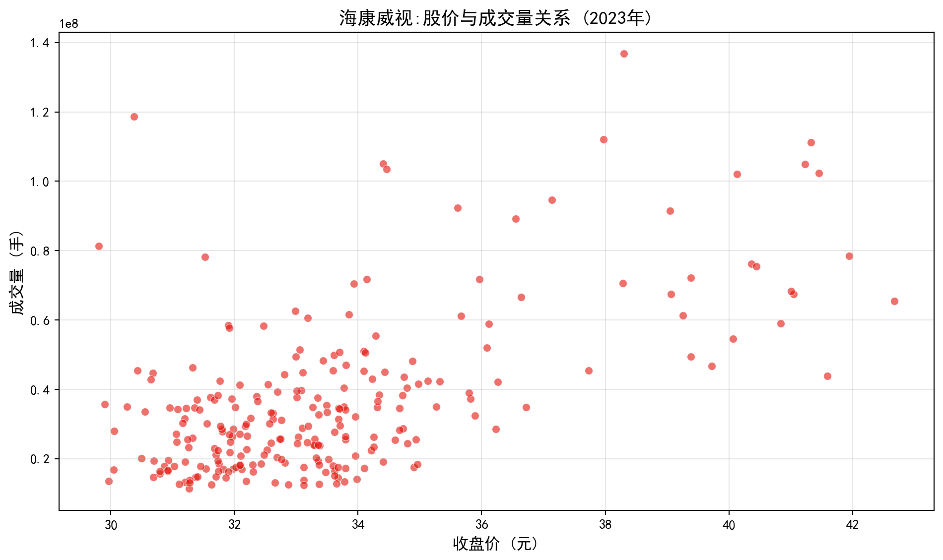
图 1.4 展示了股价与成交量的关系。从图中可以看出:
图 1.4 shows the relationship between stock price and trading volume. From the chart we can see:
当股价上涨时,成交量往往下降
这是一种负相关关系
可能的解释:股价高时,投资者观望情绪浓厚,交易减少
When the stock price rises, trading volume tends to decrease
This is a negative association
Possible explanation: When stock prices are high, investor sentiment turns cautious, and trading decreases
1.3.0.2 案例2:正相关关系 - 营业收入与净利润 (Case 2: Positive Association — Revenue vs. Net Profit)
企业的营业收入与净利润之间通常存在正相关关系:收入越高的企业,利润往往也越高(假设利润率保持相对稳定)。我们将使用中国A股上市公司的真实财务报表数据来验证这一关系。具体做法是:从本地财务数据中筛选长三角地区(上海、浙江、江苏、安徽)上市公司2023年年报数据,然后绘制营业收入与净利润的散点图。
There is usually a positive correlation between a company’s revenue and net profit: companies with higher revenue tend to have higher profits (assuming profit margins remain relatively stable). We will use real financial statement data from Chinese A-share listed companies to verify this relationship. Specifically, we will filter 2023 annual report data for YRD-region listed companies from local financial data, and then draw a scatter plot of revenue versus net profit.
# ========== 导入所需库 ==========
# ========== Import required libraries ==========
import pandas as pd          # 数据分析库
# Data analysis library
import numpy as np           # 数值计算库
# Numerical computation library
import matplotlib.pyplot as plt  # 绘图库
# Plotting library
import seaborn as sns        # 统计可视化库
# Statistical visualization library
import platform              # 平台检测库
# Platform detection library

# ========== 中文字体配置 ==========
# ========== Chinese font configuration ==========
plt.rcParams['font.sans-serif'] = ['SimHei', 'Microsoft YaHei']  # 设置中文字体
# Set Chinese fonts
plt.rcParams['axes.unicode_minus'] = False  # 解决负号显示问题
# Fix the minus sign display issue

# ========== 设置本地数据路径 ==========
# ========== Set local data paths ==========
if platform.system() == 'Windows':  # 判断当前操作系统类型
# Check the current operating system type
    data_path = 'C:/qiufei/data/stock'  # Windows 数据路径
    # Data path for Windows
else:  # Linux 系统下使用服务器数据路径
# Use server data path on Linux
    data_path = '/home/ubuntu/r2_data_mount/qiufei/data/stock'  # Linux 数据路径
    # Data path for Linux

# ========== 读取数据 ==========
# ========== Load data ==========
financial_statement_dataframe = pd.read_hdf(f'{data_path}/financial_statement.h5')  # 读取上市公司财务报表数据
# Load listed company financial statement data
stock_basic_dataframe = pd.read_hdf(f'{data_path}/stock_basic_data.h5')  # 读取上市公司基本信息
# Load listed company basic information上述代码从本地加载了两个核心数据集:financial_statement.h5 包含所有A股上市公司2005-2025年的季度财务报表数据(包括营业收入、净利润等指标);stock_basic_data.h5 包含上市公司的基本信息(股票代码、公司名称、所在省份、行业分类等)。
The above code loads two core datasets from local storage: financial_statement.h5 contains quarterly financial statement data for all A-share listed companies from 2005 to 2025 (including revenue, net profit, etc.); stock_basic_data.h5 contains basic information about listed companies (stock code, company name, province, industry classification, etc.).
下面对数据进行筛选和清洗:首先筛选2023年第四季度报告(即年报),然后限定为长三角地区的公司,最后去除营收或利润为负数或极端值的异常记录,以确保散点图的可读性。
Below we filter and clean the data: first selecting Q4 2023 reports (i.e., annual reports), then restricting to YRD-region companies, and finally removing abnormal records with negative or extreme values for revenue or profit to ensure the scatter plot’s readability.
# ========== 筛选长三角地区2023年年报数据 ==========
# ========== Filter YRD region 2023 annual report data ==========
financial_data_2023 = financial_statement_dataframe[financial_statement_dataframe['quarter'] == '2023q4'].copy()  # 筛选四季度报(年报)
# Filter Q4 reports (annual reports)
yangtze_delta_city_list = ['上海市', '浙江省', '江苏省', '安徽省']  # 长三角地区省份列表
# List of YRD provinces
target_stocks_dataframe = stock_basic_dataframe[stock_basic_dataframe['province'].isin(yangtze_delta_city_list)]  # 筛选长三角公司
# Filter YRD companies

# 合并财务数据与公司基本信息
# Merge financial data with company basic information
merged_financial_dataframe = pd.merge(financial_data_2023, target_stocks_dataframe, on='order_book_id')  # 按股票代码合并财务数据与公司信息
# Merge financial data and company info by stock code
# 筛选出收入和利润在合理范围内的非极端异常值公司进行展示,避免图像失真(营收在0到5000亿,净利润0到500亿)
# Filter companies with revenue and profit within reasonable ranges to avoid chart distortion
cleaned_financial_dataframe = merged_financial_dataframe[  # 基于营收和净利润的合理范围进行筛选
# Filter based on reasonable ranges for revenue and net profit
    (merged_financial_dataframe['revenue'] > 0) &  # 营收大于零(排除异常值)
    # Revenue greater than zero (exclude anomalies)
    (merged_financial_dataframe['revenue'] < 5e11) &  # 营收小于5000亿元(排除极端值)
    # Revenue less than 500 billion yuan (exclude extreme values)
    (merged_financial_dataframe['net_profit'] > 0) &  # 净利润大于零(排除亏损企业)
    # Net profit greater than zero (exclude loss-making companies)
    (merged_financial_dataframe['net_profit'] < 5e10)  # 净利润小于500亿元(排除极端值)
    # Net profit less than 50 billion yuan (exclude extreme values)
].copy()  # 复制筛选结果避免链式赋值警告
# Copy filtered result to avoid chained assignment warning
cleaned_financial_dataframe = cleaned_financial_dataframe.dropna(subset=['revenue', 'net_profit'])  # 剔除存在NaN的记录
# Remove records containing NaN数据筛选与清洗完成。上述代码通过多个条件(营收大于0且小于5000亿、净利润大于0且小于500亿)过滤掉了亏损企业和极端值公司。pd.merge() 函数将财务数据与公司基本信息按股票代码(order_book_id)进行合并,使我们能够同时获取每家公司的财务指标和地区信息。
Data filtering and cleaning are complete. The above code filters out loss-making companies and extreme-value companies using multiple conditions (revenue > 0 and < 500 billion, net profit > 0 and < 50 billion). The pd.merge() function merges financial data with company basic information by stock code (order_book_id), enabling us to access both financial metrics and regional information for each company.
下面使用散点图和趋势线(trend line)来可视化营业收入与净利润的关系。趋势线通过最小二乘法拟合一元线性回归得到,直观展示两个变量的线性关系方向和强度。
Below we use a scatter plot and trend line to visualize the relationship between revenue and net profit. The trend line is obtained by fitting a simple linear regression using ordinary least squares, intuitively showing the direction and strength of the linear relationship between the two variables.
# ========== 绘制散点图与趋势线 ==========
# ========== Draw scatter plot and trend line ==========
plt.figure(figsize=(10, 6))  # 创建10x6英寸画布
# Create a 10x6-inch canvas
sns.scatterplot(data=cleaned_financial_dataframe, x='revenue', y='net_profit', s=50, color='#008080', alpha=0.6)  # 绘制散点图
# Draw scatter plot

# 添加一次线性趋势线: 利用最小二乘法拟合一元线性回归
# Add a linear trend line: fit simple linear regression using least squares
trend_line_coefficients = np.polyfit(cleaned_financial_dataframe['revenue'], cleaned_financial_dataframe['net_profit'], 1)  # 拟合一次多项式系数
# Fit first-degree polynomial coefficients
trend_line_polynomial = np.poly1d(trend_line_coefficients)  # 构建多项式函数
# Build polynomial function
plt.plot(cleaned_financial_dataframe['revenue'], trend_line_polynomial(cleaned_financial_dataframe['revenue']), 'r--', linewidth=2, label='趋势线')  # 绘制红色虚线趋势线
# Draw red dashed trend line

plt.xlabel('营业收入 (元)', fontsize=12)  # X轴: 营业收入
# X-axis: Revenue
plt.ylabel('净利润 (元)', fontsize=12)  # Y轴: 净利润
# Y-axis: Net profit
plt.title('长三角上市公司营业收入与净利润关系 (2023)', fontsize=14, fontweight='bold')  # 图标题
# Chart title
plt.legend(fontsize=11)  # 显示图例
# Display legend
plt.grid(True, alpha=0.3)  # 显示网格线
# Display grid lines

plt.tight_layout()  # 自动调整布局
# Automatically adjust layout
plt.show()  # 展示图形
# Display the figure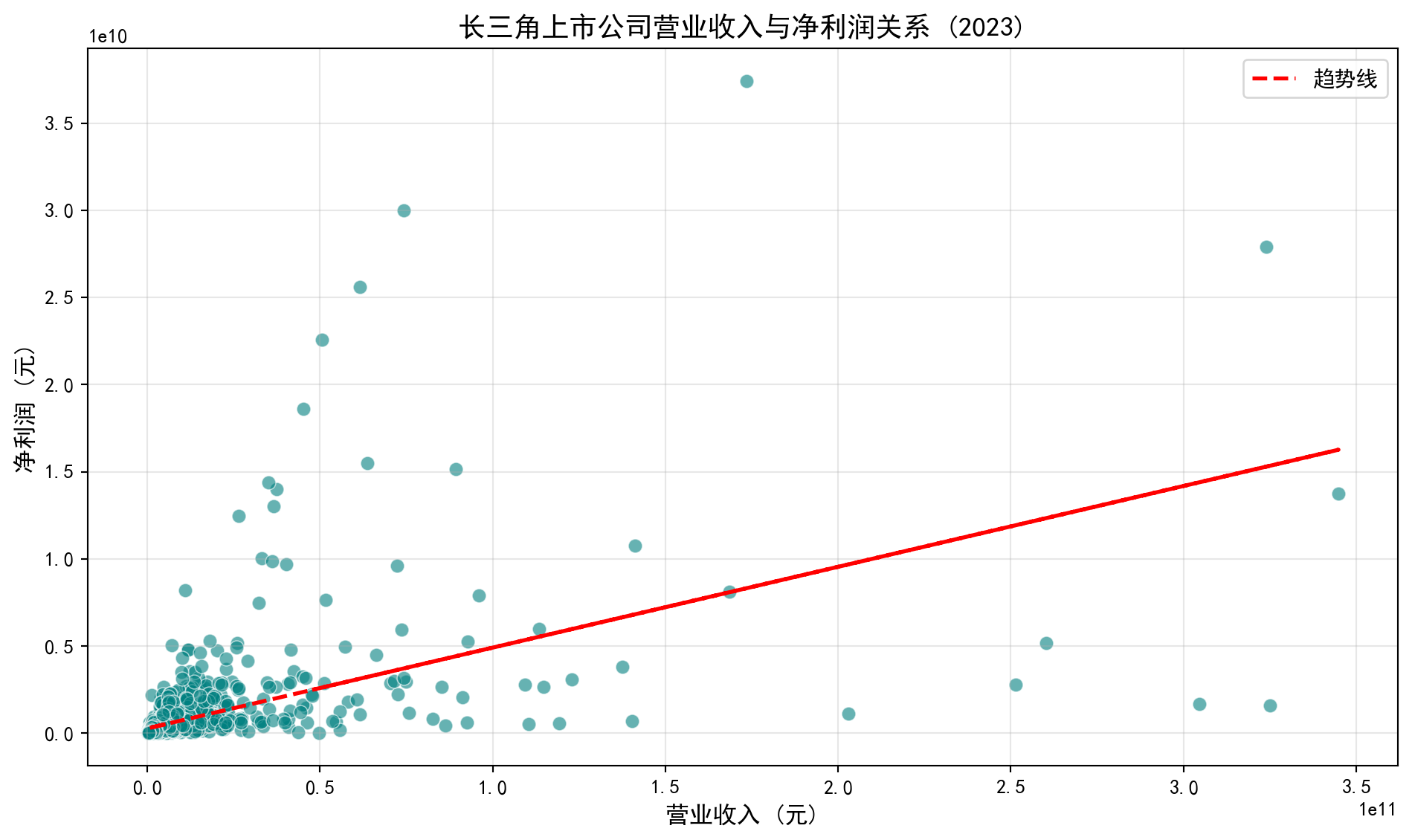
图 1.5 展示了营业收入与净利润的强正相关关系:
图 1.5 shows the strong positive correlation between revenue and net profit:
营业收入增长,净利润也随之增长
这是一种正相关关系
商业原理:在利润率保持相对稳定的情况下,企业规模的扩张往往带来绝对利润的增长
As revenue grows, net profit grows accordingly
This is a positive association
Business rationale: When profit margins remain relatively stable, expansion of firm scale generally leads to growth in absolute profit
1.3.0.3 案例3:无关联关系 - 公司注册地与ROE (Case 3: No Association — Company Location vs. ROE)
前两个案例展示了变量之间存在明确关系(正相关和负相关)的情况。然而,并非所有变量之间都存在有意义的统计关系。本案例将检验一个直觉假设:公司的注册地(分类变量)是否与其盈利能力ROE(数值变量)有关。ROE(Return on Equity,净资产收益率)是衡量企业盈利能力的核心财务指标,计算公式为:净利润 ÷ 归属母公司股东权益 × 100%。我们将从长三角四省市各取若干上市公司,比较它们的ROE分布。
The previous two cases demonstrated clear relationships (positive and negative correlations) between variables. However, not all variables have meaningful statistical relationships. This case examines an intuitive hypothesis: is a company’s registered location (categorical variable) related to its profitability ROE (numerical variable)? ROE (Return on Equity) is a core financial metric measuring corporate profitability, calculated as: Net Profit ÷ Equity Attributable to Parent Company Shareholders × 100%. We will take several listed companies from each of the four YRD provinces/municipalities and compare their ROE distributions.
# ========== 导入所需库 ==========
# ========== Import required libraries ==========
import pandas as pd          # 数据分析库
# Data analysis library
import numpy as np           # 数值计算库
# Numerical computation library
import matplotlib.pyplot as plt  # 绘图库
# Plotting library
import seaborn as sns        # 统计可视化库
# Statistical visualization library
import platform              # 平台检测库
# Platform detection library

# ========== 设置本地数据路径 ==========
# ========== Set local data paths ==========
if platform.system() == 'Windows':  # 判断当前操作系统类型
# Check the current operating system type
    data_path = 'C:/qiufei/data/stock'  # Windows 数据路径
    # Data path for Windows
else:  # Linux 系统下使用服务器数据路径
# Use server data path on Linux
    data_path = '/home/ubuntu/r2_data_mount/qiufei/data/stock'  # Linux 数据路径
    # Data path for Linux

# ========== 读取数据 ==========
# ========== Load data ==========
stock_basic_dataframe = pd.read_hdf(f'{data_path}/stock_basic_data.h5')  # 读取上市公司基本信息
# Load listed company basic information
financial_statement_dataframe = pd.read_hdf(f'{data_path}/financial_statement.h5')  # 读取财务报表数据
# Load financial statement data

# ========== 筛选长三角地区公司 ==========
# ========== Filter YRD region companies ==========
target_city_list = ['上海市', '浙江省', '江苏省', '安徽省']  # 长三角地区省份列表
# List of YRD provinces
target_stocks_dataframe = stock_basic_dataframe[stock_basic_dataframe['province'].isin(target_city_list)].head(50).copy()  # 取前50家公司
# Take the first 50 companies上述代码筛选了注册地在长三角四省市(上海、浙江、江苏、安徽)的上市公司,并取前50家作为样本。.head(50) 限制样本量是为了让散点图更清晰易读。
The above code filters listed companies registered in the four YRD provinces/municipalities (Shanghai, Zhejiang, Jiangsu, and Anhui), taking the first 50 as the sample. .head(50) limits the sample size to make the scatter plot clearer and more readable.
下面的代码从财务报表中获取每家公司最新一期的财务数据,然后计算ROE(净资产收益率)。ROE = 净利润 ÷ 归属母公司股东权益 × 100%,数值越高表示公司每投入1元股东资本能产生越多的利润。
The code below retrieves the most recent financial data for each company from financial statements, then calculates ROE (Return on Equity). ROE = Net Profit ÷ Equity Attributable to Parent Company Shareholders × 100%; a higher value indicates the company generates more profit per yuan of shareholder capital invested.
# ========== 计算ROE (净资产收益率) ==========
# ========== Calculate ROE (Return on Equity) ==========
# 获取每只股票最新季度的财务数据(按季度降序排列后去重)
# Get the most recent quarterly financial data for each stock (sort by quarter descending, then deduplicate)
latest_financial_dataframe = financial_statement_dataframe.sort_values('quarter', ascending=False).drop_duplicates('order_book_id')  # 按季度降序取每只股票最新一期数据
# Sort by quarter descending and keep only the latest record for each stock
# 计算ROE: 净利润 / 归属母公司股东权益 × 100 (转换为百分比)
# Calculate ROE: Net Profit / Equity Attributable to Parent × 100 (convert to percentage)
latest_financial_dataframe['roe'] = (  # 新增ROE列并赋值
# Add ROE column and assign values
    latest_financial_dataframe['net_profit'] / latest_financial_dataframe['equity_parent_company'] * 100  # 净利润除以归母权益再乘100转百分比
    # Net profit divided by parent equity times 100 to convert to percentage
)  # 完成ROE指标的计算赋值
# Complete the ROE calculation
# 将ROE数据合并到公司基本信息表中
# Merge ROE data into the company basic information table
merged_stock_dataframe = target_stocks_dataframe.merge(latest_financial_dataframe[['order_book_id', 'roe']], on='order_book_id', how='left')  # 左连接合并ROE数据到公司信息表
# Left join to merge ROE data into company info table
merged_stock_dataframe = merged_stock_dataframe.dropna(subset=['roe'])  # 剔除ROE为空的记录
# Remove records where ROE is null
ROE计算完成。上述代码中 .sort_values('quarter', ascending=False).drop_duplicates('order_book_id') 的作用是:对每只股票,按季度降序排列后保留第一条记录,从而获得最新一期的财务数据。.merge() 函数将ROE数据与公司基本信息合并。
ROE calculation is complete. In the above code, .sort_values('quarter', ascending=False).drop_duplicates('order_book_id') sorts each stock’s records by quarter in descending order and keeps only the first record, thereby obtaining the most recent financial data. The .merge() function combines ROE data with company basic information.
下面为各省份分配数字编码,将分类变量(省份名称)转换为数值,以便在散点图的X轴上展示。需要注意的是,这里的数字编码(0,1,2,3)仅用于绘图定位,不具有数学意义——这正是我们前面讲到的「分类变量不能进行数学运算」的例子。
Below we assign numeric codes to each province, converting the categorical variable (province name) to numerical values for display on the X-axis of the scatter plot. Note that these numeric codes (0, 1, 2, 3) are used solely for plotting positioning and carry no mathematical meaning — this is exactly the example of “categorical variables cannot be subjected to arithmetic operations” we discussed earlier.
# ========== 为城市分配数字编码(用于X轴) ==========
# ========== Assign numeric codes to cities (for X-axis) ==========
city_to_code_mapping = {city: i for i, city in enumerate(target_city_list)}  # 构建城市→数字编码映射字典
# Build city-to-numeric-code mapping dictionary
merged_stock_dataframe['city_code'] = merged_stock_dataframe['province'].map(city_to_code_mapping)  # 将省份映射为数字编码
# Map province to numeric code

# ========== 中文字体配置 ==========
# ========== Chinese font configuration ==========
plt.rcParams['font.sans-serif'] = ['SimHei', 'Microsoft YaHei']  # 设置中文字体
# Set Chinese fonts
plt.rcParams['axes.unicode_minus'] = False  # 解决负号显示问题
# Fix the minus sign display issue

# ========== 绘制散点图 ==========
# ========== Draw scatter plot ==========
plt.figure(figsize=(10, 6))  # 创建10x6英寸画布
# Create a 10x6-inch canvas
sns.scatterplot(data=merged_stock_dataframe, x='city_code', y='roe', alpha=0.6, color='#F0A700')  # 绘制散点图
# Draw scatter plot

plt.xlabel('城市编码', fontsize=12)  # X轴: 城市编码
# X-axis: City code
plt.ylabel('ROE (%)', fontsize=12)  # Y轴: 净资产收益率
# Y-axis: Return on Equity
plt.title('长三角城市与上市公司ROE关系', fontsize=14, fontweight='bold')  # 图标题
# Chart title
plt.xticks(range(len(target_city_list)), target_city_list, rotation=45)  # 将X轴刻度替换为城市名称
# Replace X-axis tick labels with city names
plt.grid(True, alpha=0.3, axis='y')  # 仅显示Y轴方向网格线
# Display only Y-axis grid lines

plt.tight_layout()  # 自动调整布局
# Automatically adjust layout
plt.show()  # 展示图形
# Display the figure
图 1.6 展示了城市与ROE之间没有明显的系统关系:
图 1.6 shows that there is no clear systematic relationship between city and ROE:
不同城市的公司ROE分布相似
这是一种无关联关系
公司的盈利能力更多取决于自身经营,而非注册地
Companies in different cities have similar ROE distributions
This is a case of no association
A company’s profitability depends more on its own operations than on its registered location
1.3.1 关联不等于因果 (Association Does Not Imply Causation)
这是统计学中最重要的原则之一,也是最容易误解的概念。
This is one of the most important principles in statistics and also one of the most easily misunderstood concepts.
1.3.1.1 经典案例:空调销量与啤酒销量 (Classic Example: Air Conditioner Sales vs. Beer Sales)
在夏季,某零售平台发现空调销量和啤酒销量同时上升。两者高度相关,但显然:
In summer, a retail platform finds that air conditioner sales and beer sales both rise simultaneously. The two are highly correlated, but obviously:
购买空调不会导致购买更多啤酒
两者的真实关系:都与夏季高温相关
高温 → 空调需求上升
高温 → 啤酒需求上升
Buying air conditioners does not cause people to buy more beer
The real relationship: both are related to summer heat
High temperature → Increased demand for air conditioners
High temperature → Increased demand for beer
这种情况下,夏季温度是一个混淆变量(confounding variable)。
In this situation, summer temperature is a confounding variable.
1.3.1.2 中国商业案例 (Chinese Business Cases)
案例1:上海房价与深圳房价 (Case 1: Shanghai Housing Prices vs. Shenzhen Housing Prices)
观察:上海房价上涨,深圳房价也上涨
相关性强,但不是因果关系
真实原因:都受宏观经济政策、流动性宽松等因素影响
Observation: When Shanghai housing prices rise, Shenzhen housing prices also rise
The correlation is strong, but it is not a causal relationship
Real reason: Both are affected by macroeconomic policies, monetary easing, and other factors
案例2:高管学历与公司绩效 (Case 2: Executive Education vs. Company Performance)
- 观察:高学历CEO的公司往往绩效更好
- 但不能简单推断:高学历 → 公司绩效好
- 可能的混淆变量:
- 高学历CEO通常在更大、更成熟的公司
- 这些公司有更好的资源和品牌
- 公司规模和成熟度才是真正的影响因素
- Observation: Companies with highly educated CEOs tend to perform better
- But one cannot simply infer: High education → Good company performance
- Possible confounding variables:
- Highly educated CEOs are typically at larger, more mature companies
- These companies have better resources and brand recognition
- Company size and maturity are the real influencing factors
建立因果关系的条件 (Conditions for Establishing Causation)
要从关联推断因果,需要满足三个条件:
To infer causation from association, three conditions must be met:
时间顺序:原因必须在结果之前
强关联:两者之间有稳定的统计关联
排除混淆:控制其他可能的解释
Temporal order: The cause must precede the effect
Strong association: There is a stable statistical association between the two
Elimination of confounding: Other possible explanations are controlled
只有通过精心设计的随机对照实验,才能可靠地建立因果关系。观察性研究无论数据多大,只能展示关联,不能证明因果。
Only through carefully designed randomized controlled experiments can causation be reliably established. Observational studies, no matter how large the data, can only show association and cannot prove causation.
1.3.2 混淆变量 (Confounding Variables)
混淆变量是与解释变量和响应变量都相关,但未被研究考虑的变量。
A confounding variable is a variable that is related to both the explanatory variable and the response variable but is not accounted for in the study.
1.3.2.1 金融案例:低市盈率与高收益 (Financial Case: Low P/E Ratio and High Returns)
观察:研究发现购买低市盈率(PE)股票的投资者往往获得更高收益。
Observation: Research finds that investors who buy low P/E ratio stocks tend to earn higher returns.
错误结论:低市盈率直接导致高收益。
Incorrect conclusion: Low P/E ratio directly causes high returns.
真实原因:低市盈率往往出现在行业景气度处于底部的公司。当行业周期反转时,盈利快速恢复推动了股价上涨。行业周期反转才是真正的因果因素,低市盈率只是行业低谷期的一种表征。
Real reason: Low P/E ratios often appear in companies whose industries are at the bottom of the business cycle. When the industry cycle reverses, rapid earnings recovery drives stock price increases. Industry cycle reversal is the true causal factor; low P/E is merely a symptom of the industry trough.
1.3.2.2 商业案例:周末购物与消费金额 (Business Case: Weekend Shopping vs. Spending Amount)
观察:周末购物的人均消费比工作日高20%。
Observation: Per capita spending on weekends is 20% higher than on weekdays.
错误结论:周末导致消费增加。
Incorrect conclusion: Weekends cause increased spending.
真实原因:周末购物者更多是全职工作者(收入更高),而工作日购物者更多是退休人员或学生。就业状态和收入是混淆变量。
Real reason: Weekend shoppers are more likely to be full-time workers (higher income), while weekday shoppers are more likely to be retirees or students. Employment status and income are confounding variables.
解决方法 (Solutions):
分层分析:分别比较全职工作者的周末vs工作日消费
多元回归:控制收入、就业状态等变量
Stratified analysis: Compare full-time workers’ weekend vs. weekday spending separately
Multiple regression: Control for income, employment status, and other variables
1.4 数据收集方法 (Data Collection Methods)
数据收集是统计分析的第一步。数据的质量直接决定了分析结果的可靠性。如果数据收集过程有偏差,再精妙的统计方法也无法得出正确结论。
Data collection is the first step of statistical analysis. The quality of data directly determines the reliability of analytical results. If the data collection process is biased, even the most sophisticated statistical methods cannot yield correct conclusions.
1.4.1 观察性研究与实验研究 (Observational Studies vs. Experimental Studies)
观察性研究(Observational Study)只是观察和记录对象的特征,不对研究对象进行干预。
An Observational Study merely observes and records the characteristics of subjects without intervening.
常见类型:
Common types:
横截面研究(Cross-sectional):在一个时间点上观察(如2023年A股上市公司的财务快照)
回顾性研究(Retrospective):回溯过去的数据(如分析2008-2023年金融危机的影响)
前瞻性研究(Prospective):跟踪一段时间(如跟踪新上市公司3年)
Cross-sectional study: Observing at a single point in time (e.g., a financial snapshot of A-share listed companies in 2023)
Retrospective study: Looking back at historical data (e.g., analyzing the impact of financial crises from 2008-2023)
Prospective study: Tracking over a period of time (e.g., following newly listed companies for 3 years)
实验研究(Experimental Study)通过主动干预来研究因果关系。
An Experimental Study investigates causal relationships through active intervention.
关键要素:
Key elements:
处理/干预(Treatment):对实验组施加的条件
对照/控制(Control):对照组不施加处理
随机化(Randomization):随机分配对象到实验组和对照组
Treatment/Intervention: The condition applied to the experimental group
Control: The control group does not receive the treatment
Randomization: Randomly assigning subjects to experimental and control groups
1.4.1.1 量化投资实验设计 (Quantitative Investment Experiment Design)
假设某基金公司想验证新开发的量化投资因子是否真的有效:
Suppose a fund company wants to verify whether a newly developed quantitative investment factor is truly effective:
研究问题:新因子模型能否提高投资组合的超额收益?
Research question: Can the new factor model improve portfolio excess returns?
实验设计:
Experiment design:
样本量:随机选取3000只A股股票
随机分配:
- 处理组:1500只股票按新因子信号构建组合
- 对照组:1500只股票按传统因子信号构建组合
双盲设计:基金经理和分析师在评估期内不知道哪组使用了新因子
主要终点:比较两组的超额收益率、夏普比率
Sample size: Randomly select 3,000 A-share stocks
Random assignment:
- Treatment group: 1,500 stocks form a portfolio based on the new factor signals
- Control group: 1,500 stocks form a portfolio based on traditional factor signals
Double-blind design: Fund managers and analysts do not know which group uses the new factor during evaluation
Primary endpoint: Compare excess returns and Sharpe ratios between the two groups
为什么需要随机化?
Why is randomization necessary?
如果不随机分配,可能出现系统偏差:
Without random assignment, systematic bias may occur:
研究人员倾向于将新因子应用于历史表现好的股票
这些股票本身就有更高的收益
无法判断是新因子有效,还是选股池本身的差异
Researchers tend to apply the new factor to stocks with good historical performance
These stocks inherently have higher returns
It becomes impossible to determine whether the new factor is effective or whether the stock pool itself differs
随机化的作用:平衡两组的已知和未知因素,确保只有”是否使用新因子”这一变量不同。
The role of randomization: Balance known and unknown factors between the two groups, ensuring that the only difference is “whether the new factor is used.”
1.4.1.2 随机区组设计 (Randomized Block Design)
当存在已知的影响因素但不是研究重点时,可以使用随机区组设计。
When there are known influencing factors that are not the focus of the study, a Randomized Block Design can be used.
中国金融案例:交易员培训方案实验
Chinese financial case: Trader training program experiment
研究问题:比较两种新的交易员培训方案(A方案:实盘模拟训练;B方案:理论案例教学)对交易绩效的影响
Research question: Compare the effects of two new trader training programs (Plan A: Live simulation training; Plan B: Theoretical case teaching) on trading performance
挑战:交易员的初始经验水平差异很大,会影响结果
Challenge: Traders’ initial experience levels vary significantly, which affects the results
解决方案:
Solution:
将交易员按从业年限分为三个区组(blocks):
- 资深交易员区组(10年以上)
- 中级交易员区组(3-10年)
- 初级交易员区组(3年以下)
在每个区组内随机分配交易员到方案A和方案B
确保每个培训方案组都有相同数量的各经验层级交易员
Divide traders into three blocks by years of experience:
- Senior trader block (10+ years)
- Intermediate trader block (3-10 years)
- Junior trader block (under 3 years)
Randomly assign traders within each block to Plan A and Plan B
Ensure each training program group has equal numbers of traders from each experience level
优势:
Advantages:
控制了初始经验水平的影响
提高了实验的统计功效(statistical power)
可以检验培训方案是否对不同经验层级的交易员有不同效果(交互效应)
Controls the effect of initial experience level
Improves the statistical power of the experiment
Can test whether the training program has different effects on traders at different experience levels (interaction effect)
1.5 抽样方法 (Sampling Methods)
1.5.1 总体、样本与统计推断 (Population, Sample, and Statistical Inference)
在统计学中:
In statistics:
总体(Population):研究对象的全体
样本(Sample):从总体中抽取的、用于研究的较小子集
参数(Parameter):总体特征,用希腊字母表示(如总体均值\(\mu\))
统计量(Statistic):样本特征,用普通字母表示(如样本均值\(\bar{x}\))
Population: The entire group of subjects under study
Sample: A smaller subset drawn from the population for study
Parameter: A population characteristic, denoted by Greek letters (e.g., population mean \(\mu\))
Statistic: A sample characteristic, denoted by ordinary letters (e.g., sample mean \(\bar{x}\))
案例:
Example:
总体:所有中国A股上市公司(约5000家)
样本:被抽取研究的100家公司
参数:所有公司的平均市盈率(P/E ratio)
统计量:这100家公司的平均市盈率
Population: All Chinese A-share listed companies (approximately 5,000)
Sample: 100 companies selected for study
Parameter: The average P/E ratio of all companies
Statistic: The average P/E ratio of these 100 companies
1.5.1.1 为什么需要抽样? (Why Is Sampling Necessary?)
进行全面调查(普查)往往不现实:
Conducting a complete census is often impractical:
- 成本太高:调查全部5000家上市公司需要巨大人力物力
- 时间太长:等到调查完成,情况可能已经变化
- 破坏性测试:某些测试是破坏性的,不能对全部对象进行
- 案例:测试灯泡寿命,必须用到灯泡烧毁
- 不能测试所有灯泡,否则就没有产品可卖了
- Too costly: Surveying all 5,000 listed companies requires enormous human and material resources
- Too time-consuming: By the time the survey is complete, conditions may have changed
- Destructive testing: Some tests are destructive and cannot be performed on all subjects
- Example: Testing light bulb lifespan requires burning them out
- You cannot test all light bulbs, otherwise there would be none left to sell
1.5.1.2 统计推断的核心思想 (The Core Idea of Statistical Inference)
关键问题:如何从100家样本公司的市盈率,推断全部5000家公司的市盈率?
Key question: How can we infer the P/E ratio of all 5,000 companies from the P/E ratio of 100 sample companies?
统计推断的答案:
The answer from statistical inference:
样本是总体的代表(如果抽样得当)
样本统计量是总体参数的估计
通过置信区间(confidence interval)量化估计的不确定性
通过假设检验(hypothesis testing)判断结论的可靠性
The sample represents the population (if properly sampled)
Sample statistics are estimates of population parameters
Confidence intervals quantify the uncertainty of estimates
Hypothesis testing assesses the reliability of conclusions
我们将在第5章详细学习这些方法。
We will study these methods in detail in Chapter 5.
1.5.2 简单随机抽样 (Simple Random Sampling)
定义:每个个体被抽中的概率相等,且每个可能的样本被抽中的概率也相等。
Definition: Every individual has an equal probability of being selected, and every possible sample has an equal probability of being selected.
案例:中国消费者信心调查
Example: Chinese Consumer Confidence Survey
假设要从上海2000万成年人中抽取1500人进行消费者信心调查:
Suppose we want to sample 1,500 people from Shanghai’s 20 million adults for a consumer confidence survey:
实施方法:
Implementation method:
获得上海所有成年人的抽样框
使用计算机随机数生成器
随机抽取1500人
确保每个人被抽中的概率相等
Obtain a sampling frame of all adults in Shanghai
Use a computer random number generator
Randomly select 1,500 people
Ensure each person has an equal probability of being selected
挑战:
Challenges:
抽样框不完整:某些人群可能不在抽样框中(如无固定电话者)
无响应偏差:被抽中的人可能拒绝参与调查
Incomplete sampling frame: Some groups may not be in the sampling frame (e.g., those without landline phones)
Nonresponse bias: Selected individuals may refuse to participate
1.5.3 抽样偏差 (Sampling Bias)
抽样偏差是系统性误差,不同于数据的自然变异,无法通过统计技术修正。
Sampling bias is a systematic error, different from natural data variability, and cannot be corrected by statistical techniques.
1.5.3.1 常见类型 (Common Types)
选择偏差(Selection Bias)
案例:在写字楼里进行的消费调查
Example: Consumer survey conducted in office buildings
问题:会高估收入水平(白领集中)
被抽取的样本不能代表整个人群
Problem: Overestimates income level (concentration of white-collar workers)
The sample drawn cannot represent the entire population
自愿响应偏差(Voluntary Response Bias)
案例:网络投票、微博热搜调查
Example: Online polls, Weibo trending-topic surveys
- 问题:只能吸引持有强烈观点的人参与
- 历史教训:
- 1948年美国总统大选,电话民意测验预测杜威获胜
- 但实际杜鲁门获胜
- 原因:当时只有富裕家庭(支持杜威)有电话
- Problem: Attracts only those with strong opinions
- Historical lesson:
- In the 1948 U.S. presidential election, telephone polls predicted Dewey would win
- But Truman actually won
- Reason: At the time, only wealthy families (who supported Dewey) had telephones
无响应偏差(Nonresponse Bias)
案例:邮寄问卷回收率低
Example: Low return rate for mailed questionnaires
问题:响应者可能与不响应者有系统性差异
比如年轻人更不愿意回复纸质问卷
Problem: Responders may systematically differ from non-responders
For example, young people are less willing to reply to paper questionnaires
幸存者偏差 (Survivorship Bias):二战飞机的启示
(Survivorship Bias: Lessons from World War II Aircraft)
这是统计学历史上最著名的反例之一,由统计学家亚伯拉罕·沃德 (Abraham Wald) 在二战期间提出。
This is one of the most famous counterexamples in the history of statistics, proposed by statistician Abraham Wald during World War II.
现象:返航的战机上,机翼被打得千疮百孔,而驾驶舱和引擎完好无损。
军方直觉:应该加强机翼的装甲,因为那里弹孔最多。
统计学家直觉:错!应该加强驾驶舱和引擎。
Observation: Returning aircraft had wings riddled with bullet holes, while cockpits and engines were intact.
Military intuition: Reinforce the wing armor, because that’s where most bullet holes are.
Statistician’s intuition: Wrong! Reinforce the cockpit and engine.
逻辑:
Logic:
我们只能看到返航的飞机(幸存者)。
那些驾驶舱和引擎中弹的飞机,根本就没能飞回来(被样本剔除了)。
机翼上的弹孔反而证明了:即使机翼中弹,飞机依然能活下来。
We can only see the aircraft that returned (survivors).
Those aircraft hit in the cockpit and engine never made it back (they were excluded from the sample).
Bullet holes in the wings actually prove that: even if the wings are hit, the plane can still survive.
主要启示:数据分析最危险的不是数据里有什么,而是数据里缺了什么。在商业中,我们分析成功的公司(幸存者),试图总结”成功经验”,却往往忽略了那些做了同样事情但破产了的公司。
Key takeaway: The most dangerous thing in data analysis is not what is in the data, but what is missing from the data. In business, we analyze successful companies (survivors) and try to summarize “success factors,” but often overlook companies that did the same things but went bankrupt.
1.5.4 中国民意调查的挑战 (Challenges of Public Opinion Polling in China)
2016年美国总统大选的预测失败是统计学界的经典案例。许多民调机构错误预测希拉里获胜,原因是:
The failure to predict the 2016 U.S. presidential election is a classic case in the statistics community. Many polling organizations incorrectly predicted Hillary Clinton would win, because:
错过了新增的”特朗普选民”
抽样框未能充分覆盖农村地区
响应率低,且特朗普支持者更不愿意参与调查
They missed the new “Trump voters”
The sampling frame failed to adequately cover rural areas
Response rates were low, and Trump supporters were less willing to participate in surveys
中国类似的挑战:
Similar challenges in China:
城乡差异
(Urban-rural divide)
一线城市调查结果不能代表全国
农村地区的消费习惯、价值观与城市差异很大
First-tier city survey results cannot represent the entire country
Rural areas’ consumption habits and values differ greatly from cities
数字鸿沟
(Digital divide)
网络调查会漏掉不使用互联网的群体
老年人、农村居民、低收入者被低估
Online surveys miss groups that do not use the internet
The elderly, rural residents, and low-income individuals are underrepresented
地域文化差异
(Regional cultural differences)
长三角的消费习惯可能与西北地区完全不同
全国性调查需要确保地域代表性
Consumption habits in the Yangtze River Delta may be completely different from the Northwest
National surveys need to ensure regional representativeness
政治敏感性
(Political sensitivity)
某些敏感话题的调查可能得到不真实的回答
社会期望偏差(Social Desirability Bias):受访者按照”社会期望”而非真实想法回答
Surveys on certain sensitive topics may receive untruthful responses
Social Desirability Bias: Respondents answer according to “social expectations” rather than their true thoughts
1.5.5 其他抽样方法 (Other Sampling Methods)
虽然本教材主要使用简单随机抽样,但实践中还有其他专门方法:
Although this textbook primarily uses simple random sampling, there are other specialized methods used in practice:
分层抽样(Stratified Sampling)
先将总体分成若干层(strata)
再从每层随机抽样
案例:按省份分层,确保每个省份都有足够样本
First divide the population into several strata
Then randomly sample from each stratum
Example: Stratify by province to ensure each province has an adequate sample
整群抽样(Cluster Sampling)
将总体分成若干群
随机抽取部分群
调查群内所有个体
案例:随机抽取若干个学校,调查这些学校的所有学生
优势:节省成本,不需要跑遍全国
Divide the population into several clusters
Randomly select some clusters
Survey all individuals within the selected clusters
Example: Randomly select several schools and survey all students in those schools
Advantage: Saves cost, no need to travel nationwide
1.5.6 3. 系统抽样 (Systematic Sampling)
按固定间隔抽取
案例:从生产线上每隔100件产品抽取1件检验
实施简单,但要注意周期性模式
Select at fixed intervals
Example: Inspect 1 product for every 100 on the production line
Simple to implement, but watch out for periodic patterns
1.6 从理论到实践:苦活累活 (From Theory to Practice: The “Dirty Work”)
每一本统计学教科书在介绍方法时,通常都假设数据是完美的:没有缺失值,没有录入错误,样本完美代表总体。然而,现实世界的数据是”脏乱”的。在应用任何统计模型之前,数据科学家往往要花80%的时间进行数据清洗和预处理。
Every statistics textbook, when introducing methods, typically assumes that the data is perfect: no missing values, no entry errors, and samples perfectly represent the population. However, real-world data is “messy.” Before applying any statistical model, data scientists often spend 80% of their time on data cleaning and preprocessing.
1.6.1 数据质量陷阱 (Data Quality Traps)
即使是像上市公司财务报表这样经过审计的数据,也并非完美无缺。
Even audited data such as listed company financial statements is not flawless.
缺失值 (Missing Values): 公司可能因为停牌、推迟披露年报等原因导致数据缺失。
异常值 (Outliers): 录入错误或极端事件(如巨额亏损)会导致某些指标偏离正常范围几个数量级。
幸存者偏差 (Survivorship Bias): 这是金融数据分析中最危险的陷阱。
Missing Values: Companies may have missing data due to trading suspensions, delayed annual reports, etc.
Outliers: Entry errors or extreme events (such as massive losses) can cause certain metrics to deviate several orders of magnitude from normal ranges.
Survivorship Bias: This is the most dangerous trap in financial data analysis.
让我们通过一个实际的 Python 案例来演示什么是幸存者偏差。
Let us demonstrate survivorship bias through a practical Python example.
1.6.2 案例研究:幸存者偏差的验证 (Case Study: Verifying Survivorship Bias)
很多关于”长期投资”的研究会告诉你:如果你在10年前买入A股所有股票并持有至今,平均收益率是多少。但这些研究往往犯了一个致命错误:它们只统计了现在还活着的公司。
Many studies on “long-term investing” will tell you: what would the average return be if you had bought all A-share stocks 10 years ago and held them until now. But these studies often make a fatal error: they only count companies that are still alive today.
事实上,有很多公司在过去10年里因为业绩不佳而退市了。如果我们只分析现在的上市公司,就人为地剔除了那些”失败者”,从而高估了市场的平均表现。
In fact, many companies were delisted over the past 10 years due to poor performance. If we only analyze currently listed companies, we artificially exclude those “losers,” thereby overestimating the market’s average performance.
让我们用本地的 stock_basic 数据来看看,到底有多少公司”消失”了。
Let us use local stock_basic data to see how many companies have “disappeared.”
# ========== 导入所需库 ==========
# ========== Import required libraries ==========
import pandas as pd   # 数据分析库
# Data analysis library
import platform       # 平台检测库
# Platform detection library

# ========== 设置本地数据路径 ==========
# ========== Set local data paths ==========
if platform.system() == 'Windows':  # 判断当前操作系统类型
# Check the current operating system type
    data_path = 'C:/qiufei/data/stock'  # Windows 数据路径
    # Data path for Windows
else:  # Linux 系统下使用服务器数据路径
# Use server data path on Linux
    data_path = '/home/ubuntu/r2_data_mount/qiufei/data/stock'  # Linux 数据路径
    # Data path for Linux

# ========== 读取并分析数据 ==========
# ========== Load and analyze data ==========
stock_basic_dataframe = pd.read_hdf(f'{data_path}/stock_basic_data.h5')  # 读取上市公司基本信息
# Load listed company basic information

# 统计各上市状态的公司数量: Active(上市)、Delisted(退市)、Unknown(暂停上市)
# Count companies by listing status: Active (Listed), Delisted, Unknown (Paused)
listing_status_counts = stock_basic_dataframe['status'].value_counts()  # 按上市状态分组计数
# Group and count by listing status
# 将英文状态名替换为中英文对照的标签
# Replace English status names with bilingual labels
status_name_mapping = {'Active': '上市 (Listed)', 'Delisted': '退市 (Delisted)', 'Unknown': '暂停上市 (Paused)'}  # 定义英文到中英文对照的映射
# Define mapping from English to bilingual labels
listing_status_counts.index = listing_status_counts.index.map(status_name_mapping)  # 应用映射替换索引标签
# Apply mapping to replace index labels

# ========== 输出统计结果 ==========
# ========== Output statistical results ==========
print("中国A股上市公司状态统计:")  # 打印统计结果标题
# Print the title of statistical results
print(listing_status_counts)  # 输出各状态公司数量
# Output the number of companies in each status

# 计算退市公司在全部公司中的占比
# Calculate the proportion of delisted companies among all companies
delisted_company_ratio = listing_status_counts['退市 (Delisted)'] / listing_status_counts.sum()  # 退市数量除以总数得到退市比例
# Divide delisted count by total to get delisted ratio
print(f"\n历史上有 {delisted_company_ratio:.1%} 的公司已经退市。")  # 以百分比格式输出退市比率
# Output delisted ratio in percentage format
print("如果在回测策略时忽略了这些公司,你的策略收益率将被显著高估。")  # 提示幸存者偏差对回测的影响
# Warn about the impact of survivorship bias on backtesting
中国A股上市公司状态统计:
status
上市 (Listed) 5183
退市 (Delisted) 320
暂停上市 (Paused) 21
Name: count, dtype: int64
历史上有 5.8% 的公司已经退市。
如果在回测策略时忽略了这些公司,你的策略收益率将被显著高估。这就是“苦活累活”:在跑模型之前,你必须先检查数据的完整性,思考数据生成过程中是否存在偏差。如果数据本身就是有偏的(如幸存者偏差),那么无论你的统计模型多么高深,得出的结论都是错误的(Garbage In, Garbage Out)。
This is the “dirty work”: before running models, you must first check data integrity and consider whether bias exists in the data generation process. If the data itself is biased (such as survivorship bias), then no matter how sophisticated your statistical model is, the conclusions will be wrong (Garbage In, Garbage Out).
1.7 本书的路线图 (Roadmap of This Book)
在开始详细学习之前,让我们先通过 图 1.7 一览全书的知识架构和学习路径。
Before diving into the details, let us first take a bird’s-eye view of the entire book’s knowledge architecture and learning path through 图 1.7.
1.7.1 第一部分:描述统计学 (Part I: Descriptive Statistics)
第2章:描述性数据分析 (Chapter 2: Descriptive Data Analysis)
本章将介绍描述统计的主要方法:
This chapter introduces the main methods of descriptive statistics:
- 集中趋势的度量:均值、中位数、众数
- 离散程度的度量:方差、标准差、四分位距、变异系数
- 分布形状的度量:偏度、峰度
- 数据可视化:直方图、箱线图、散点图、条形图
描述统计的目标是描述手头的样本,而不对样本来源的更大总体进行推断。这就像是给数据拍照片,记录它的特征。
The goal of descriptive statistics is to describe the sample at hand, without making inferences about the larger population from which the sample was drawn. It is like taking a photograph of the data, recording its characteristics.
1.7.2 第二部分:概率基础 (Part II: Probability Foundations)
第3章:概率基础 (Chapter 3: Probability Foundations)
本章介绍统计学所需的概率理论:
This chapter introduces the probability theory required for statistics:
- 概率的定义和基本性质
- 条件概率与独立性
- 全概率公式与贝叶斯定理
- 计数原理:排列与组合
第4章:概率分布 (Chapter 4: Probability Distributions)
本章介绍统计学中最重要的概率分布:
This chapter introduces the most important probability distributions in statistics:
- 离散分布:二项分布、泊松分布、几何分布
- 连续分布:正态分布、指数分布、均匀分布
- 抽样分布:正态分布、t分布、卡方分布、F分布
这些内容是推断统计的理论基础。理解概率分布,就像理解物理定律一样,是构建统计推断方法的前提。
These topics form the theoretical foundation of inferential statistics. Understanding probability distributions, much like understanding the laws of physics, is a prerequisite for constructing statistical inference methods.
1.7.3 第三部分:推断统计 (Part III: Inferential Statistics)
第5-9章:推断统计的核心方法 (Chapters 5-9: Core Methods of Inferential Statistics)
第5章:推断统计基础 (Chapter 5: Foundations of Inferential Statistics)
- 点估计与区间估计
- 置信区间的构建与解释
- 假设检验的基本思想
- 比例的检验(单样本、两样本)
第6章:拟合优度与独立性检验 (Chapter 6: Goodness-of-Fit and Independence Tests)
- 拟合优度检验:观察分布是否符合理论分布
- 列联表与独立性检验:两个分类变量是否相关
- 适合性检验的实际应用
第7章:均值推断 (Chapter 7: Inference for Means)
- 单样本t检验
- 两独立样本t检验
- 配对样本t检验
- 单因素方差分析(ANOVA)
第8章:相关与回归 (Chapter 8: Correlation and Regression)
- 相关系数:Pearson、Spearman
- 简单线性回归:最小二乘法
- 回归诊断:残差分析、异常值检测
- 预测与解释
第9章:方差分析(ANOVA) (Chapter 9: Analysis of Variance)
- 单因素ANOVA
- 多重比较问题
- 双因素ANOVA:交互效应
- 方差分析的假设与诊断
推断统计使用样本统计量对总体参数进行推断,就像是根据样本推测总体。这是统计学从”描述过去”到”预测未来”的飞跃。
Inferential statistics uses sample statistics to make inferences about population parameters, essentially inferring the whole from a part. This represents a leap in statistics from “describing the past” to “predicting the future.”
1.7.4 第四部分:高级方法 (Part IV: Advanced Methods)
第10-13章:现代数据分析方法 (Chapters 10-13: Modern Data Analysis Methods)
第10章:多元模型 (Chapter 10: Multivariate Models)
- 多元线性回归
- 变量选择方法
- 多重共线性问题
- 交互效应与非线性变换
第11章:非线性模型 (Chapter 11: Nonlinear Models)
- 多项式回归
- 分段回归
- 广义线性模型(GLM):Logistic回归、Poisson回归
- 正则化方法:Ridge、Lasso
第12章:基于树的方法 (Chapter 12: Tree-Based Methods)
- 决策树:分类树与回归树
- 集成方法:Bagging、随机森林
- Boosting:AdaBoost、Gradient Boosting
- XGBoost在中国金融科技中的应用
第13章:无监督模型 (Chapter 13: Unsupervised Models)
- 主成分分析(PCA):数据降维
- 因子分析:发现潜在因子
- 聚类分析:K-means、层次聚类
- 客户细分在电商中的应用
这些方法在现代商业数据分析、机器学习中有广泛应用。阿里巴巴、拼多多、携程等互联网公司大量使用这些方法进行个性化推荐、风险控制、用户画像等。
These methods are widely used in modern business data analytics and machine learning. Internet companies such as Alibaba, Pinduoduo, and Ctrip extensively employ these methods for personalized recommendations, risk management, user profiling, and more.
1.8 统计学在中国商业中的应用 (Applications of Statistics in Chinese Business)
统计学在中国经济发展中扮演着越来越重要的角色。以下是一些典型应用场景:
Statistics plays an increasingly important role in China’s economic development. The following are some typical application scenarios:
1.8.1 金融市场 (Financial Markets)
量化投资 (Quantitative Investment):
- 使用统计模型构建交易策略
- 因子投资:发现能预测股票收益的因子
- 中证金工:中国量化基金的管理规模超过1万亿元
风险管理 (Risk Management):
- VaR(在险价值)模型:评估最大可能损失
- 压力测试:极端情况下的风险暴露
- 信用风险模型:违约概率(PD)、违约损失率(LGD)
案例:国泰君安使用蒙特卡洛模拟计算投资组合风险,每日VaR模型帮助控制风险暴露。
Case study: Guotai Junan Securities uses Monte Carlo simulation to calculate portfolio risk, with daily VaR models helping to control risk exposure.
1.8.2 电子商务 (E-commerce)
推荐系统 (Recommendation Systems):
- 协同过滤算法:阿里”猜你喜欢”
- 基于内容的推荐:苏宁易购商品推荐
- 深度学习推荐:淘宝个性化推荐
A/B测试 (A/B Testing):
- 美团:优化外卖配送算法
- 拼多多:测试不同的营销策略
- 抖音:优化视频推荐机制
用户画像 (User Profiling):
- 基于统计的用户细分
- 客户生命周期价值(CLV)预测
- 流失预警模型
1.8.3 保险与风控 (Insurance and Risk Control)
精算定价 (Actuarial Pricing):
- 车险、寿险、健康险的风险定价模型
- 基于GLM(广义线性模型)的费率厘定
- 太平洋保险的智能核保系统:利用统计模型实现自动化风险评估
信用风险管理 (Credit Risk Management):
- 信用评分卡(Scorecard):利用Logistic回归对借款人违约概率建模
- 蚂蚁金服的芝麻信用评分体系
- 商业银行不良贷款率预测
反欺诈检测 (Anti-Fraud Detection):
- 异常交易识别:基于统计异常检测算法
- 保险理赔欺诈的统计特征分析
- 实时交易监控中的假设检验应用
1.8.4 政府决策 (Government Decision-Making)
经济指标 (Economic Indicators):
- CPI:居民消费价格指数
- GDP:国内生产总值
- PMI:采购经理指数
政策评估 (Policy Evaluation):
- 使用因果推断方法评估政策效果
- 双重差分(DID)模型
- 倾向得分匹配(PSM)
人口普查 (Census):
- 大规模数据的收集和分析
- 抽样设计
- 数据质量评估
1.9 本章小结 (Chapter Summary)
本章介绍了统计学的基本概念和思维方式:
This chapter introduced the fundamental concepts and ways of thinking in statistics:
核心概念 (Core Concepts):
统计学的价值:从不确定的数据中提取有价值的信息
变量类型:数值变量(离散、连续)和分类变量(名义、有序)
变量关系:正相关、负相关、无关联;关联不等于因果
混淆变量:导致虚假关联的第三方变量
The value of statistics: Extracting valuable information from uncertain data
Variable types: Numerical variables (discrete, continuous) and categorical variables (nominal, ordinal)
Variable relationships: Positive correlation, negative correlation, no association; association does not equal causation
Confounding variables: Third-party variables that lead to spurious associations
数据收集 (Data Collection):
研究方法:观察性研究(只能展示关联)vs实验研究(可以建立因果)
抽样方法:简单随机抽样、避免抽样偏差
实验设计:对照、随机化、重复、双盲
Research methods: Observational studies (can only show association) vs. experimental studies (can establish causation)
Sampling methods: Simple random sampling, avoiding sampling bias
Experimental design: Control, randomization, replication, double-blinding
统计思维 (Statistical Thinking):
不确定性:习惯用概率而非确定性思考
变异:数据总是有变异,这是自然的
推断:从样本到总体需要量化不确定性
Uncertainty: Getting accustomed to thinking in probabilities rather than certainties
Variation: Data always has variation — this is natural
Inference: Going from sample to population requires quantifying uncertainty
统计学不仅仅是计算公式和编程技术,更是一种科学思维方法。在后续章节中,我们将系统学习统计学的理论、方法和应用,最终目标是让读者能够:
Statistics is not merely about formulas and programming techniques; it is a scientific way of thinking. In the following chapters, we will systematically study statistical theory, methods, and applications, with the ultimate goal of enabling readers to:
从数据中发现规律和洞见
做出基于证据的决策
量化决策的不确定性
在商业实践中应用统计方法
Discover patterns and insights from data
Make evidence-based decisions
Quantify the uncertainty of decisions
Apply statistical methods in business practice
1.10 思考与练习 (Exercises and Reflections)
1.10.1 概念理解 (Conceptual Understanding)
1. 变量类型识别 (Variable Type Identification)
识别以下变量的类型,并说明理由:
Identify the type of each variable below, and explain your reasoning:
- 中国A股上市公司的市值
- 消费者的满意度评分(1-5星)
- 公司的注册地(省份)
- 每月的交易天数
- 员工的工号
- 手机号码
- 每日登录次数
- 网页加载时间(秒)
2. 研究类型判断 (Research Type Classification)
判断以下研究是观察性研究还是实验研究,并说明原因:
Determine whether each of the following studies is observational or experimental, and explain why:
- 研究高负债与企业破产的关系:调查1000家ST企业和1000家正常企业的财务指标
- 测试新教学方法的效果:随机分配学生到新方法和传统方法组
- 分析GDP与股市表现的关系:收集10年GDP和股指数据
- 比较两种营销策略的效果:在不同城市使用不同策略
- 研究广告投入与销售增长的关系:跟踪500家企业5年的广告支出和营收数据
3. 混淆变量识别 (Confounding Variable Identification)
识别以下情境中可能的混淆变量:
Identify possible confounding variables in each of the following scenarios:
- 发现常去健身房的人收入更高
- 发现使用iPhone的人更愿意购买高端产品
- 发现大学毕业生收入更高
- 发现拥有更多信用卡的人信用评分更高
- 发现广告投入更多的企业品牌知名度更高
1.10.2 实际应用 (Practical Applications)
4. 案例分析:微信支付 vs 支付宝支付 (Case Study: WeChat Pay vs. Alipay)
假设一项研究发现:微信支付用户的平均交易金额比支付宝用户高20%。
Suppose a study finds: The average transaction amount of WeChat Pay users is 20% higher than that of Alipay users.
问题 (Questions):
- 这个发现能说明”使用微信支付导致消费增加”吗?为什么?
Can this finding demonstrate that “using WeChat Pay causes increased spending”? Why or why not?
- 可能有哪些混淆变量?
What possible confounding variables might exist?
- 应该如何设计研究来建立因果关系?
How should a study be designed to establish a causal relationship?
- 如果要你进行一个A/B测试,你会如何设计?
If you were to conduct an A/B test, how would you design it?
5. 研究设计:在线教育效果 (Research Design: Online Education Effectiveness)
要评估在线教育相比传统课堂教育的效果,应该如何设计实验?
To evaluate the effectiveness of online education compared to traditional classroom education, how should the experiment be designed?
问题 (Questions):
- 需要控制哪些变量?
What variables need to be controlled?
- 如何避免可能的偏差?
How can potential biases be avoided?
- 应该使用什么指标来衡量”效果”?
What metrics should be used to measure “effectiveness”?
- 样本量应该多大?为什么?
How large should the sample size be? Why?
6. 抽样方案设计 (Sampling Plan Design)
要调查某品牌电动汽车(如蔚来、小鹏)的用户满意度:
To investigate user satisfaction with a specific brand of electric vehicle (e.g., NIO, XPeng):
问题 (Questions):
- 目标总体是什么?
What is the target population?
- 应该如何抽样?
How should sampling be conducted?
- 可能遇到哪些偏差?如何避免?
What biases might be encountered? How can they be avoided?
- 应该调查多少人?为什么?
How many people should be surveyed? Why?
1.10.3 数据分析 (Data Analysis)
7. 本地数据获取与分析 (Local Data Retrieval and Analysis)
使用本地股票数据完成以下任务:
Use local stock data to complete the following tasks:
import pandas as pd
import matplotlib.pyplot as plt
import platform

# 设置数据路径
# Set data path
if platform.system() == 'Windows':
    data_path = 'C:/qiufei/data/stock'
else:
    data_path = '/home/ubuntu/r2_data_mount/qiufei/data/stock'

# 读取本地数据
# Read local data
stock_basic = pd.read_hdf(f'{data_path}/stock_basic_data.h5')
stock_price = pd.read_hdf(f'{data_path}/stock_price_pre_adjusted.h5')
stock_price = stock_price.reset_index()

# 任务1:选择5家长三角地区上市公司
# Task 1: Select 5 listed companies from the Yangtze River Delta region
# 提示:筛选stock_basic的area字段
# Hint: Filter the area field of stock_basic

# 任务2:获取这些公司2023年的日收益率数据
# Task 2: Get the daily return data for these companies in 2023
# 提示:从stock_price筛选后计算收益率
# Hint: Filter from stock_price and then calculate returns

# 任务3:计算相关系数矩阵
# Task 3: Compute the correlation coefficient matrix
# 提示:使用DataFrame.corr()方法
# Hint: Use the DataFrame.corr() method

# 任务4:绘制散点图矩阵
# Task 4: Plot a scatter plot matrix
# 提示:使用pd.plotting.scatter_matrix()
# Hint: Use pd.plotting.scatter_matrix()
8. 公司财务分析 (Company Financial Analysis)
获取某公司(如海康威视002415.XSHE)的历史数据:
Retrieve historical data for a company (e.g., Hikvision 002415.XSHE):
# 任务1:从stock_price中筛选2023年日度行情数据
# Task 1: Filter 2023 daily market data from stock_price
# 提示:筛选order_book_id和日期范围
# Hint: Filter by order_book_id and date range

# 任务2:计算日收益率
# Task 2: Calculate daily returns
# 提示:使用np.log()计算对数收益率
# Hint: Use np.log() to calculate log returns

# 任务3:绘制收盘价与成交量的散点图
# Task 3: Plot a scatter chart of closing price vs. volume
# 任务4:判断是正相关、负相关还是无关联
# Task 4: Determine whether the relationship is positive, negative, or no association
# 任务5:添加趋势线(使用numpy.polyfit())
# Task 5: Add a trend line (using numpy.polyfit())
9. 数据框操作 (DataFrame Operations)
创建一个包含以下信息的数据框:
Create a DataFrame containing the following information:
10家上市公司
变量:公司名称、股票代码、所属行业、注册地、2023年营收、员工数量
10 listed companies
Variables: company name, stock code, industry, registered location, 2023 revenue, number of employees
然后 (Then):
- 计算数值变量的描述统计
Calculate descriptive statistics for numerical variables
- 按行业分组,计算平均营收
Group by industry and calculate average revenue
- 筛选出营收超过1000亿元的公司
Filter companies with revenue exceeding 100 billion yuan
- 创建新的比率变量:人均营收
Create a new ratio variable: revenue per employee
1.10.4 深度思考 (Deep Thinking)
10. 因果关系的哲学思考 (Philosophical Reflections on Causality)
- 为什么观察性研究不能建立因果关系?
Why can’t observational studies establish causal relationships?
- 什么情况下可以从关联推断因果?
Under what circumstances can causation be inferred from association?
- “因果”的定义是什么?是哲学问题还是科学问题?
What is the definition of “causation”? Is it a philosophical question or a scientific one?
- 在商业决策中,为什么区分关联和因果如此重要?
In business decision-making, why is distinguishing between association and causation so important?
11. 大数据时代的统计推断 (Statistical Inference in the Big Data Era)
- 在大数据时代,为什么还需要抽样?
In the big data era, why is sampling still needed?
- 什么情况下可以使用全量数据?
Under what circumstances can the entire dataset be used?
- 当n=100万时,微小的差异也会统计显著,这带来了什么问题?
When n = 1 million, even tiny differences become statistically significant — what problems does this create?
- “统计显著”等于”实际重要”吗?为什么?
Does “statistically significant” equal “practically important”? Why or why not?
12. 数据伦理 (Data Ethics)
- A/B测试是否需要告知用户他们正在被测试?
Should users be informed that they are being tested in an A/B test?
- 如果实验组获得更好的待遇,这符合伦理吗?
If the treatment group receives better treatment, is this ethical?
- 如何平衡科学研究和用户权益?
How can scientific research and user rights be balanced?
- 举例说明数据滥用可能带来的危害
Give examples of the potential harm caused by data misuse
1.10.5 挑战性题目 (Challenge Problems)
13. 设计一个完整的商业实验 (Design a Complete Business Experiment)
选择一个你感兴趣的商业场景,设计一个完整的随机对照实验:
Choose a business scenario that interests you and design a complete randomized controlled experiment:
场景示例 (Example scenarios):
- 测试新的APP界面设计
- 评估不同的定价策略
- 比较广告文案的效果
- 测试新的推荐算法
要求 (Requirements):
- 明确研究问题
Define the research question clearly
- 定义响应变量
Define the response variable
- 设计实验方案
Design the experimental protocol
- 确定样本量
Determine the sample size
- 说明如何随机化
Explain how randomization will be implemented
- 预期结果和商业意义
Expected results and business implications
14. 批判性分析 (Critical Analysis)
阅读一篇商业新闻或研究报告,分析其中:
Read a business news article or research report and analyze:
- 数据来源是否可靠?
Is the data source reliable?
- 样本是否具有代表性?
Is the sample representative?
- 是否存在混淆变量?
Do confounding variables exist?
- 结论是否恰当?
Is the conclusion appropriate?
- 你会如何改进这项研究?
How would you improve this study?
15. 实证验证:幸存者偏差的影响 (Empirical Verification: The Impact of Survivorship Bias)
这是一个稍微复杂但极具启发性的练习。我们将量化忽略退市公司会造成多大的误差。
This is a slightly complex but highly insightful exercise. We will quantify how much error is introduced by ignoring delisted companies.
import pandas as pd
import numpy as np

# 步骤1:获取2015年1月1日之前上市的所有公司代码
# Step 1: Get all company codes listed before January 1, 2015
# 提示:筛选 listed_date < '2015-01-01'
# Hint: Filter listed_date < '2015-01-01'

# 步骤2:分别计算两组公司的"平均ROE"(或其他财务指标)
# Step 2: Calculate the "average ROE" (or other financial metrics) for two groups
# 组A (幸存者):至今仍在上市的公司 (status='Active')
# Group A (survivors): Companies still listed today (status='Active')
# 组B (失败者):后来退市的公司 (status='Delisted')
# Group B (failures): Companies that were subsequently delisted (status='Delisted')

# 提示:
# Hints:
# - 使用 stock_basic 数据获取名单
# - Use stock_basic data to get the list
# - 使用 financial_statement 数据获取 2014 年年报的 ROE
# - Use financial_statement data to get ROE from the 2014 annual report
# - 比较两组 ROE 的均值
# - Compare the mean ROE of the two groups

# 问题:
# Questions:
# (1) 退市组在退市前的财务表现是否已经显著差于幸存组?
# (1) Was the financial performance of the delisted group already significantly worse than the survivor group before delisting?
# (2) 如果我们在2015年初构建投资组合,若只看现在的数据库(可能已剔除退市公司),
#     我们会看到什么样的虚假繁荣?
# (2) If we constructed a portfolio in early 2015, and only looked at the current database (which may have removed delisted companies),
#     what kind of false prosperity would we see?
1.10.6 参考答案 (Reference Answers)
习题 1.1 解答 (Solution to Exercise 1.1)
| 变量 (Variable) | 变量类型 (Type) | 理由 (Reasoning) |
|---|---|---|
| 中国A股上市公司的市值 | 连续型数值变量 | 市值可以取任何正实数值(如1.23亿、456.78亿),具有大小和比值意义 |
| Market capitalization of A-share listed companies | Continuous numerical variable | Market cap can take any positive real value (e.g., 123 million, 45.678 billion), with meaningful magnitude and ratio |
| 消费者的满意度评分(1-5星) | 有序分类变量 | 虽用数字表示,但等级间距不必等距,加减运算无意义(“非常好”减”一般”≠“好”) |
| Consumer satisfaction rating (1-5 stars) | Ordinal categorical variable | Although represented by numbers, the intervals between levels are not necessarily equal; arithmetic operations are meaningless |
| 公司的注册地(省份) | 名义分类变量 | 省份名称是无序的类别标签,无法比较大小 |
| Company registered location (province) | Nominal categorical variable | Province names are unordered category labels; they cannot be compared in magnitude |
| 每月的交易天数 | 离散型数值变量 | 交易天数只能取非负整数值(0, 1, 2, …),是可计数的 |
| Monthly trading days | Discrete numerical variable | Trading days can only take non-negative integer values (0, 1, 2, …); they are countable |
| 员工的工号 | 名义分类变量 | 工号虽为数字,但仅用作标识,加减乘除无实际意义 |
| Employee ID number | Nominal categorical variable | Although numeric, ID numbers serve only as identifiers; arithmetic operations have no practical meaning |
| 手机号码 | 名义分类变量 | 手机号虽为数字,但仅用作标识,数学运算(如两人手机号求平均)无任何意义 |
| Phone number | Nominal categorical variable | Although numeric, phone numbers serve only as identifiers; mathematical operations (e.g., averaging two phone numbers) are meaningless |
| 每日登录次数 | 离散型数值变量 | 登录次数只能取非负整数值(0, 1, 2, …),是可计数的 |
| Daily login count | Discrete numerical variable | Login counts can only take non-negative integer values (0, 1, 2, …); they are countable |
| 网页加载时间(秒) | 连续型数值变量 | 加载时间可以取任意非负实数值(如0.35秒、2.718秒),具有大小和比例意义 |
| Web page loading time (seconds) | Continuous numerical variable | Loading time can take any non-negative real value (e.g., 0.35s, 2.718s), with meaningful magnitude and ratio |
关键辨析要点:区分数值变量和分类变量的核心标准不在于变量”是否由数字表示”,而在于其数值运算是否有实际意义。工号”001”和”002”相加等于”003”毫无意义,所以工号是分类变量;而市值100亿和200亿相加等于300亿是有意义的,所以市值是数值变量。
Key Distinction: The core criterion for distinguishing numerical variables from categorical variables is not whether the variable “is represented by numbers,” but whether arithmetic operations on those numbers are meaningful. Adding employee IDs “001” and “002” to get “003” is meaningless, so employee ID is a categorical variable; adding market caps of 10 billion and 20 billion to get 30 billion is meaningful, so market cap is a numerical variable.
习题 1.2 解答 (Solution to Exercise 1.2)
研究吸烟与肺癌的关系:观察性研究(回顾性)。研究者并未主动干预让受试者吸烟,只是被动观察已有病史。
Studying the relationship between smoking and lung cancer: Observational study (retrospective). The researchers did not actively intervene by making subjects smoke; they only passively observed existing medical histories.
测试新教学方法的效果:实验研究。研究者主动实施了干预(分配教学方法),并使用了随机化,符合随机对照实验的特征。
Testing the effectiveness of a new teaching method: Experimental study. The researchers actively implemented an intervention (assigning teaching methods) and used randomization, meeting the characteristics of a randomized controlled experiment.
分析GDP与股市表现的关系:观察性研究(回顾性/历史数据)。研究者仅收集历史数据,无法对国家GDP或股市进行人为操纵。
Analyzing the relationship between GDP and stock market performance: Observational study (retrospective/historical data). Researchers only collected historical data and could not artificially manipulate national GDP or the stock market.
比较两种营销策略的效果:实验研究(A/B 测试)。研究者主动在不同城市实施不同策略来观察效果。如果在选择城市时进行了随机分配,这是典型的现场实验。
Comparing the effectiveness of two marketing strategies: Experimental study (A/B test). Researchers actively implemented different strategies in different cities to observe outcomes. If cities were randomly assigned, this is a typical field experiment.
研究广告投入与销售增长的关系:观察性研究(前瞻性/队列研究)。研究者只能长期跟踪企业的自然广告支出和营收变化,无法强制企业未来5年的广告投放策略。
Studying the relationship between advertising spending and sales growth: Observational study (prospective/cohort study). Researchers can only track companies’ natural advertising expenditures and revenue changes over time; they cannot dictate a company’s advertising strategy for the next 5 years.
习题 1.3 解答 (Solution to Exercise 1.3)
混淆变量:社会经济地位/空闲时间。收入更高的人通常有更多时间、金钱和精力去健身房。
Confounding variable: Socioeconomic status / leisure time. People with higher incomes typically have more time, money, and energy to go to the gym.
混淆变量:收入水平。iPhone 用户往往平均收入偏高,所以能负担得起其他高端产品。
Confounding variable: Income level. iPhone users tend to have higher average incomes, so they can afford other premium products.
混淆变量:家庭背景/先天智力/勤奋程度。这些因素既增加了上大学的概率,也决定了未来的收入。
Confounding variable: Family background / innate intelligence / diligence. These factors both increase the probability of attending college and determine future income.
混淆变量:收入水平/消费习惯。拥有更多信用卡的人通常经济活动更活跃、收入更高,而这些因素本身就会提高信用评分。
Confounding variable: Income level / spending habits. People with more credit cards typically have more active economic lives and higher incomes, and these factors themselves raise credit scores.
混淆变量:企业规模/市场地位。广告投入更多的企业往往本身就是行业龙头,拥有更强的品牌基础和市场占有率,即使不做广告知名度也很高。
Confounding variable: Company size / market position. Companies that spend more on advertising tend to be industry leaders with stronger brand foundations and market share; their brand awareness would be high even without advertising.
习题 1.4 解答 (Solution to Exercise 1.4)
不能说明”使用微信支付导致消费增加”。研究发现的仅仅是相关性(association),而非因果关系(causation)。微信支付用户平均交易金额高20%这一事实,可能由多种其他因素解释,平台选择本身不一定是消费金额差异的原因。这是典型的”相关不等于因果”(correlation does not imply causation)的案例。
It cannot demonstrate that “using WeChat Pay causes increased spending.” The finding merely shows association, not causation. The fact that WeChat Pay users have a 20% higher average transaction amount may be explained by many other factors; the choice of platform itself may not be the cause of the spending difference. This is a classic case of “correlation does not imply causation.”
可能的混淆变量包括:
Possible confounding variables include:
- 用户年龄与收入:微信的用户群可能覆盖更多中高收入的中青年群体,而收入水平直接影响消费金额。
- User age and income: WeChat’s user base may include more middle-to-high income young and middle-aged users, and income level directly affects spending amounts.
- 消费场景差异:微信支付在高端商超、线下门店等场景中的渗透率可能更高,而支付宝在电商平台小额消费中使用更频繁。
- Differences in consumption scenarios: WeChat Pay may have higher penetration in high-end supermarkets and brick-and-mortar stores, while Alipay is used more frequently for small online purchases.
- 地域差异:一线城市用户可能更倾向于使用微信支付,而一线城市的物价和消费水平本就更高。
- Regional differences: Users in first-tier cities may prefer WeChat Pay, and prices and consumption levels in first-tier cities are inherently higher.
- 用户使用习惯:部分用户可能习惯将大额消费放在微信支付,小额消费使用支付宝,导致观测到的差异。
- User habits: Some users may habitually use WeChat Pay for large purchases and Alipay for small ones, leading to the observed difference.
建立因果关系的研究设计:
Research designs to establish causation:
- 随机对照实验(RCT):招募一批此前同时使用两种支付方式的消费者,随机将他们分为两组,一组仅使用微信支付,另一组仅使用支付宝,在一段固定时间后比较两组的平均交易金额。
- Randomized Controlled Trial (RCT): Recruit consumers who previously used both payment methods, randomly divide them into two groups — one using only WeChat Pay, the other only Alipay — and compare average transaction amounts after a fixed period.
- 准实验方法:利用某些”自然实验”情境(如某商场突然只支持微信支付),采用双重差分法(Difference-in-Differences)比较政策变化前后两组消费者的消费变化。
- Quasi-experimental methods: Use “natural experiment” situations (e.g., a mall suddenly only supporting WeChat Pay), applying Difference-in-Differences to compare spending changes before and after the policy change.
- 倾向值匹配(Propensity Score Matching):在观察性数据中,先根据年龄、收入、地域等变量进行匹配,使两组用户的特征尽可能相似,再比较消费差异。
- Propensity Score Matching (PSM): In observational data, first match users based on variables such as age, income, and region to make the two groups as similar as possible, then compare spending differences.
A/B测试设计方案:
A/B test design:
- 参与者招募:从某电商或零售平台招募自愿参与者,要求他们同时绑定了微信支付和支付宝账户。
- Participant recruitment: Recruit voluntary participants from an e-commerce or retail platform, requiring that they have both WeChat Pay and Alipay accounts linked.
- 随机分组:将参与者随机分入实验组(默认支付方式设为微信支付)和对照组(默认支付方式设为支付宝),注意需保证两组在年龄、性别、历史消费金额等关键维度上分布均衡。
- Random assignment: Randomly assign participants to the treatment group (default payment set to WeChat Pay) and control group (default payment set to Alipay), ensuring balanced distribution across key dimensions such as age, gender, and historical spending.
- 实验周期:持续4-8周,以消除短期波动效应。
- Experiment duration: 4-8 weeks, to eliminate short-term fluctuation effects.
- 观测指标:主要指标为人均交易金额;辅助指标包括交易频次、单笔最大金额、活跃天数等。
- Metrics: Primary metric is per-capita transaction amount; secondary metrics include transaction frequency, maximum single transaction amount, active days, etc.
- 统计检验:对两组人均交易金额进行独立样本 \(t\) 检验(或在样本量较大时使用非参数检验),检验显著性水平设为 \(\alpha = 0.05\)。
- Statistical testing: Conduct an independent-sample \(t\)-test on per-capita transaction amounts (or use a nonparametric test for large samples), with significance level set at \(\alpha = 0.05\).
习题 1.5 解答 (Solution to Exercise 1.5)
在线教育效果实验设计:
Experimental design for online education effectiveness:
控制变量:学生的初始水平(可通过随机区组设计控制)、年龄、性别、学习时长、网络条件等。
Control variables: students’ initial proficiency (can be controlled through randomized block design), age, gender, study duration, internet conditions, etc.
避免偏差:确保两组的内容难度一致;使用标准化客观考试衡量效果以避免主观偏差。
Bias avoidance: Ensure content difficulty is consistent for both groups; use standardized objective exams to measure effectiveness to avoid subjective bias.
衡量指标:期末考试的最终分数,或干预前后的分数增量差异(Difference-in-Differences)。
Metrics: Final exam scores, or pre-post score differences (Difference-in-Differences).
样本量:需做统计效力分析(Power Analysis),一般需要足够大(如每组至少几百人)以抹平个体自然差异,确保大数定律生效,并且足以检测到具有实际意义的最小效果。
Sample size: A power analysis is needed; generally, the sample should be large enough (e.g., at least several hundred per group) to smooth out individual natural differences, ensure the law of large numbers takes effect, and detect the minimum effect of practical significance.
习题 1.6 解答 (Solution to Exercise 1.6)
电动汽车满意度抽样设计:
Sampling design for electric vehicle satisfaction:
目标总体:所有购买并正在使用该品牌电动汽车的用户。
Target population: All users who have purchased and are currently using that brand of electric vehicle.
抽样方法:可以采用系统抽样(基于车架号间隔)或分层抽样(按省份、车型分层后再随机抽样)。
Sampling method: Systematic sampling (based on VIN intervals) or stratified sampling (stratified by province and model, then random sampling within strata).
偏差与避免:无响应偏差(仅极度满意或极度不满意的用户更愿意填表)。缓解方法:给予一定物质奖励以提升普通用户的回复率;或采用电话回访等强制力更强的回访方法。
Bias and avoidance: Non-response bias (only extremely satisfied or extremely dissatisfied users are more willing to fill out surveys). Mitigation: Offer material incentives to boost response rates among average users; or use more proactive follow-up methods such as phone callbacks.
样本量规模:取决于你能容忍的最大误差范围和置信水平(见后续章节的推断统计样本量规划),一般需要几百上千人。
Sample size: Depends on the maximum margin of error and confidence level you can tolerate (see sample size planning in later chapters on inferential statistics); generally, several hundred to a thousand people are needed.
习题 1.7 解答 (Solution to Exercise 1.7)
本题要求选择5家长三角地区上市公司,获取2023年日收益率数据并计算相关系数矩阵。解题思路分三步:(1) 从本地数据中筛选长三角地区上市公司并选取5家;(2) 获取这5家公司2023年全年的日度行情数据,计算日收益率;(3) 基于收益率数据计算Pearson相关系数矩阵,分析公司间的联动关系。
This exercise requires selecting 5 listed companies from the Yangtze River Delta region, obtaining their 2023 daily return data, and calculating the correlation coefficient matrix. The approach involves three steps: (1) filter Yangtze Delta listed companies from local data and select 5; (2) obtain full-year 2023 daily market data for these 5 companies and calculate daily returns; (3) calculate the Pearson correlation coefficient matrix based on the return data to analyze inter-company co-movements.
# ========== 导入所需库 ==========
# ========== Import required libraries ==========
import pandas as pd       # 数据处理与分析
# Data processing and analysis
import numpy as np        # 数值计算
# Numerical computation
import matplotlib.pyplot as plt  # 绘图库
# Plotting library
import platform           # 操作系统检测
# Operating system detection

# ========== 中文字体配置 ==========
# ========== Chinese font configuration ==========
plt.rcParams['font.sans-serif'] = ['SimHei', 'Microsoft YaHei']  # 设置中文字体
# Set Chinese font
plt.rcParams['axes.unicode_minus'] = False  # 解决负号显示问题
# Fix minus sign display issue

# ========== 第1步:设置本地数据路径(跨平台兼容) ==========
# ========== Step 1: Set local data path (cross-platform compatible) ==========
if platform.system() == 'Windows':  # 判断当前操作系统类型
    # Determine the current operating system
    data_path = 'C:/qiufei/data/stock'   # Windows 平台数据路径
    # Windows platform data path
else:  # Linux 系统下使用服务器数据路径
    # Use server data path on Linux
    data_path = '/home/ubuntu/r2_data_mount/qiufei/data/stock'  # Linux 平台数据路径
    # Linux platform data path

# ========== 第2步:读取本地数据 ==========
# ========== Step 2: Read local data ==========
stock_basic_dataframe = pd.read_hdf(f'{data_path}/stock_basic_data.h5')  # 上市公司基本信息
# Listed company basic information
stock_price_dataframe = pd.read_hdf(f'{data_path}/stock_price_pre_adjusted.h5')  # 前复权日度行情
# Pre-adjusted daily market data
stock_price_dataframe = stock_price_dataframe.reset_index()  # 将索引列转为普通列,方便后续筛选
# Convert index to regular columns for easier filtering
本地数据读取完毕。下面筛选长三角地区上市公司并输出分析结果。
Local data loaded. Next, we filter Yangtze Delta listed companies and output the analysis results.
# ========== 第3步(任务1):选择5家长三角地区上市公司 ==========
# ========== Step 3 (Task 1): Select 5 Yangtze Delta listed companies ==========
yangtze_province_list = ['上海市', '浙江省', '江苏省']  # 长三角三省一市(此处取三省市)
# Yangtze Delta provinces (three provinces/municipalities selected here)
# 筛选省份在长三角范围内的公司,取前5家
# Filter companies whose province is within the Yangtze Delta, take the first 5
yangtze_target_stocks = stock_basic_dataframe[stock_basic_dataframe['province'].isin(yangtze_province_list)].head(5)  # 筛选长三角地区公司并取前5家
# Filter Yangtze Delta companies and take the first 5
selected_stock_codes = yangtze_target_stocks['order_book_id'].tolist()  # 提取股票代码列表
# Extract the list of stock codes

# 输出选取结果
# Output the selection results
print('=' * 60)  # 打印分隔线
# Print separator line
print('习题1.7解答:长三角上市公司分析')  # 打印标题
# Print title
print('=' * 60)  # 打印分隔线
# Print separator line
print(f'\n任务1:选择的5家长三角公司')  # 输出任务1标题
# Output Task 1 heading
print(yangtze_target_stocks[['order_book_id', 'abbrev_symbol', 'province', 'industry_name']].to_string(index=False))  # 输出公司信息表格(不显示行索引)
# Output company information table (without row index)
============================================================
习题1.7解答:长三角上市公司分析
============================================================
任务1:选择的5家长三角公司
order_book_id abbrev_symbol province industry_name
000035.XSHE ZGTY 江苏省 生态保护和环境治理业
000156.XSHE HSCM 浙江省 广播、电视、电影和影视录音制作业
000301.XSHE DFSH 江苏省 化学纤维制造业
000411.XSHE YTJT 浙江省 批发业
000418.XSHE XTEA 江苏省 未知5家长三角上市公司选取完成。下面获取它们2023年的日收益率并计算相关系数矩阵。
Selection of 5 Yangtze Delta listed companies completed. Next, we obtain their 2023 daily returns and calculate the correlation coefficient matrix.
# ========== 第4步(任务2):获取2023年日收益率 ==========
# ========== Step 4 (Task 2): Get 2023 daily returns ==========
# 筛选选定股票在2023年的行情数据
# Filter market data for the selected stocks in 2023
filtered_price_dataframe = stock_price_dataframe[  # 基于布尔索引筛选目标股票和日期范围
    # Filter target stocks and date range using boolean indexing
    (stock_price_dataframe['order_book_id'].isin(selected_stock_codes)) &  # 股票代码在选定列表中
    # Stock code is in the selected list
    (stock_price_dataframe['date'] >= '2023-01-01') &  # 日期不早于2023年1月1日
    # Date no earlier than January 1, 2023
    (stock_price_dataframe['date'] <= '2023-12-31')  # 日期不晚于2023年12月31日
    # Date no later than December 31, 2023
].copy()  # 复制数据避免 SettingWithCopyWarning
# Copy data to avoid SettingWithCopyWarning

# 数据透视:将长表转为宽表,每列为一只股票的收盘价序列
# Pivot: Convert long table to wide table, each column is one stock's closing price series
pivoted_price_dataframe = filtered_price_dataframe.pivot(index='date', columns='order_book_id', values='close')  # 数据透视为宽格式
# Pivot to wide format
# 计算简单日收益率(百分比变化)并去除首行NaN
# Calculate simple daily returns (percentage change) and remove first row NaN
daily_returns_dataframe = pivoted_price_dataframe.pct_change().dropna()  # 计算日简单收益率并删除缺失值
# Calculate daily simple returns and drop missing values

# 输出日收益率的描述性统计
# Output descriptive statistics of daily returns
print(f'\n任务2:日收益率统计')  # 输出任务2标题
# Output Task 2 heading
print(f'交易日数: {len(daily_returns_dataframe)}')  # 输出有效交易日总数
# Output total number of valid trading days
print(f'收益率描述统计:')  # 描述性统计提示
# Descriptive statistics prompt
print(daily_returns_dataframe.describe().round(4))  # 输出均值、标准差、四分位数等统计量
# Output mean, standard deviation, quartiles, and other statistics

# ========== 第5步(任务3):计算并输出相关系数矩阵 ==========
# ========== Step 5 (Task 3): Calculate and output correlation coefficient matrix ==========
print(f'\n任务3:相关系数矩阵')  # 输出任务3标题
# Output Task 3 heading
correlation_matrix = daily_returns_dataframe.corr()  # Pearson相关系数矩阵
# Pearson correlation coefficient matrix
print(correlation_matrix.round(3))  # 保留3位小数输出相关系数矩阵
# Output correlation coefficient matrix rounded to 3 decimal places
任务2:日收益率统计
交易日数: 241
收益率描述统计:
order_book_id  000035.XSHE  000156.XSHE  000301.XSHE  000411.XSHE
count             241.0000     241.0000     241.0000     241.0000
mean               -0.0001       0.0002      -0.0011      -0.0000
std                 0.0167       0.0200       0.0165       0.0206
min                -0.0355      -0.0754      -0.0484      -0.0876
25%                -0.0123      -0.0122      -0.0108      -0.0107
50%                -0.0017       0.0000      -0.0017       0.0000
75%                 0.0075       0.0117       0.0053       0.0092
max                 0.0649       0.0727       0.0998       0.1001

任务3:相关系数矩阵
order_book_id  000035.XSHE  000156.XSHE  000301.XSHE  000411.XSHE
order_book_id
000035.XSHE          1.000        0.058        0.277        0.177
000156.XSHE          0.058        1.000       -0.100        0.100
000301.XSHE          0.277       -0.100        1.000        0.115
000411.XSHE 0.177 0.100 0.115 1.000运行结果解读:上述代码输出了两部分关键结果。第一部分(日收益率描述统计)显示:2023年共有241个有效交易日,4只股票的日均收益率均接近零(-0.11% 至 +0.02%),这符合股票短期收益率围绕零值波动的典型特征;标准差(波动率)在1.65%至2.06%之间,表明这些中小市值股票的日内波动幅度较为接近。最小值和最大值分别约为 -8.76% 和 +10.01%,显示出个别交易日出现了较大的价格跳动(涨停或跌停附近)。第二部分(相关系数矩阵)显示:000035.XSHE 与 000301.XSHE 的相关系数最高(0.277),说明这两只股票的日收益率存在一定的正相关(同涨同跌倾向);而 000156.XSHE 与 000301.XSHE 的相关系数为负(-0.100),说明它们之间存在微弱的反向联动。大部分股票对之间的相关系数在 0.05 至 0.28 之间,总体上相关性不强,这恰恰体现了分散化投资降低风险的理论基础——选择低相关性的资产组合,可以有效降低投资组合的整体波动。
Interpretation of results: The code above outputs two key sets of results. Part 1 (Daily return descriptive statistics) shows: there are 241 valid trading days in 2023, with average daily returns for the 4 stocks all close to zero (-0.11% to +0.02%), consistent with the typical characteristic of short-term stock returns fluctuating around zero; standard deviations (volatility) range from 1.65% to 2.06%, indicating that these small-to-mid-cap stocks have similar intraday volatility. Minimum and maximum values are approximately -8.76% and +10.01% respectively, showing that individual trading days experienced large price jumps (near limit-up or limit-down). Part 2 (Correlation matrix) shows: the highest correlation is between 000035.XSHE and 000301.XSHE (0.277), indicating some positive correlation in daily returns (tendency to rise and fall together); while 000156.XSHE and 000301.XSHE have a negative correlation (-0.100), indicating weak inverse co-movement. Most stock pairs have correlations between 0.05 and 0.28, with overall weak correlations — this precisely reflects the theoretical foundation of diversified investing to reduce risk: selecting a portfolio of assets with low correlations can effectively reduce overall portfolio volatility.
习题 1.8 解答 (Solution to Exercise 1.8)
本题要求选择一家中国上市公司,将其股价与成交量的关系用散点图展示,并拟合趋势线判断相关方向。我们选择海康威视(002415.XSHE)作为分析对象,使用2023年全年前复权日度行情数据。解题步骤:(1) 筛选海康威视2023年行情数据;(2) 计算对数日收益率;(3) 绘制股价-成交量散点图并添加线性趋势线。
This exercise requires selecting a Chinese listed company, displaying the relationship between its stock price and trading volume using a scatter plot, and fitting a trend line to determine the direction of correlation. We select Hikvision (002415.XSHE) as the analysis subject, using full-year 2023 pre-adjusted daily market data. Steps: (1) filter Hikvision 2023 market data; (2) calculate log daily returns; (3) plot a price-volume scatter chart and add a linear trend line.
# ========== 导入所需库 ==========
# ========== Import required libraries ==========
import pandas as pd       # 数据处理与分析
# Data processing and analysis
import numpy as np        # 数值计算(对数收益率)
# Numerical computation (log returns)
import matplotlib.pyplot as plt  # 绘图库
# Plotting library
import seaborn as sns     # 高级可视化库(散点图)
# Advanced visualization library (scatter plots)
import platform           # 操作系统检测
# Operating system detection

# ========== 中文字体配置 ==========
# ========== Chinese font configuration ==========
plt.rcParams['font.sans-serif'] = ['SimHei', 'Microsoft YaHei']  # 设置中文字体
# Set Chinese font
plt.rcParams['axes.unicode_minus'] = False  # 解决负号显示问题
# Fix minus sign display issue

# ========== 第1步:设置本地数据路径(跨平台兼容) ==========
# ========== Step 1: Set local data path (cross-platform compatible) ==========
if platform.system() == 'Windows':  # 判断当前操作系统类型
    # Determine the current operating system
    data_path = 'C:/qiufei/data/stock'   # Windows 平台数据路径
    # Windows platform data path
else:  # Linux 系统下使用服务器数据路径
    # Use server data path on Linux
    data_path = '/home/ubuntu/r2_data_mount/qiufei/data/stock'  # Linux 平台数据路径
    # Linux platform data path

# ========== 第2步:读取行情数据 ==========
# ========== Step 2: Read market data ==========
stock_price_dataframe = pd.read_hdf(f'{data_path}/stock_price_pre_adjusted.h5')  # 前复权日度行情
# Pre-adjusted daily market data
stock_price_dataframe = stock_price_dataframe.reset_index()  # 索引转为普通列
# Convert index to regular columns
前复权行情数据读取完毕。下面筛选海康威视2023年数据并计算对数日收益率。
Pre-adjusted market data loaded. Next, we filter Hikvision 2023 data and calculate log daily returns.
# ========== 第3步(任务1&2):筛选海康威视2023年数据并计算对数收益率 ==========
# ========== Step 3 (Tasks 1&2): Filter Hikvision 2023 data and calculate log returns ==========
hikvision_price_dataframe = stock_price_dataframe[  # 基于布尔条件筛选海康威视2023年行情
    # Filter Hikvision 2023 market data using boolean conditions
    (stock_price_dataframe['order_book_id'] == '002415.XSHE') &  # 海康威视股票代码
    # Hikvision stock code
    (stock_price_dataframe['date'] >= '2023-01-01') &            # 2023年起始日
    # Start date of 2023
    (stock_price_dataframe['date'] <= '2023-12-31')              # 2023年截止日
    # End date of 2023
].copy()  # 复制数据避免链式赋值警告
# Copy data to avoid chained assignment warning
hikvision_price_dataframe = hikvision_price_dataframe.sort_values('date')  # 按日期升序排列
# Sort by date in ascending order
# 计算对数收益率:ln(今日收盘价 / 昨日收盘价)
# Calculate log returns: ln(today's close / yesterday's close)
hikvision_price_dataframe['log_return'] = np.log(hikvision_price_dataframe['close'] / hikvision_price_dataframe['close'].shift(1))  # 计算每日对数收益率
# Calculate daily log returns
hikvision_price_dataframe = hikvision_price_dataframe.dropna()  # 删除首行NaN
# Drop the first row NaN
海康威视数据加载与对数收益率计算完成。下面绘制股价-成交量散点图并拟合趋势线,完成习题1.8的综合分析。
Hikvision data loading and log return calculation complete. Next, we plot the price-volume scatter chart with a fitted trend line, completing the comprehensive analysis for Exercise 1.8.
# ========== 第4步(任务3&4&5):绘制股价-成交量散点图与趋势线 ==========
# ========== Step 4 (Tasks 3&4&5): Plot price-volume scatter chart with trend line ==========
plt.figure(figsize=(10, 6))  # 设置画布大小
# Set canvas size
# 绘制散点图:x轴为收盘价,y轴为成交量
# Plot scatter chart: x-axis is closing price, y-axis is trading volume
sns.scatterplot(data=hikvision_price_dataframe, x='close', y='volume', color='#008080')

# 用一次多项式拟合趋势线(线性拟合)
# Fit a first-degree polynomial trend line (linear fit)
trend_line_coefficients = np.polyfit(hikvision_price_dataframe['close'], hikvision_price_dataframe['volume'], 1)  # 最小二乘法拟合一次多项式系数
# Least squares fit for first-degree polynomial coefficients
trend_line_polynomial = np.poly1d(trend_line_coefficients)  # 构造多项式函数
# Construct polynomial function
# 绘制红色虚线趋势线
# Plot red dashed trend line
plt.plot(hikvision_price_dataframe['close'], trend_line_polynomial(hikvision_price_dataframe['close']), 'r--', label='趋势线')  # 绘制拟合的线性趋势线
# Plot the fitted linear trend line

# 设置图表标签和标题
# Set chart labels and title
plt.xlabel('收盘价 (元)')       # x轴标签
# x-axis label
plt.ylabel('成交量 (手)')       # y轴标签
# y-axis label
plt.title('海康威视: 股价与成交量关系 (2023)')  # 图标题
# Chart title
plt.legend()                    # 显示图例
# Show legend
plt.grid(True, alpha=0.3)       # 添加半透明网格线
# Add semi-transparent grid lines
plt.show()                      # 渲染并展示图形
# Render and display the figure

# 分析结论:多数情况下股票呈现价升量增的正相关,或因观望而形成负相关。
# Analytical conclusion: In most cases stocks show positive correlation of rising price with increasing volume, or negative correlation due to wait-and-see sentiment.
# 图中可直观看出关系并不绝对,需视股价所处阶段而定。
# The chart shows intuitively that the relationship is not absolute and depends on the stage of the stock price.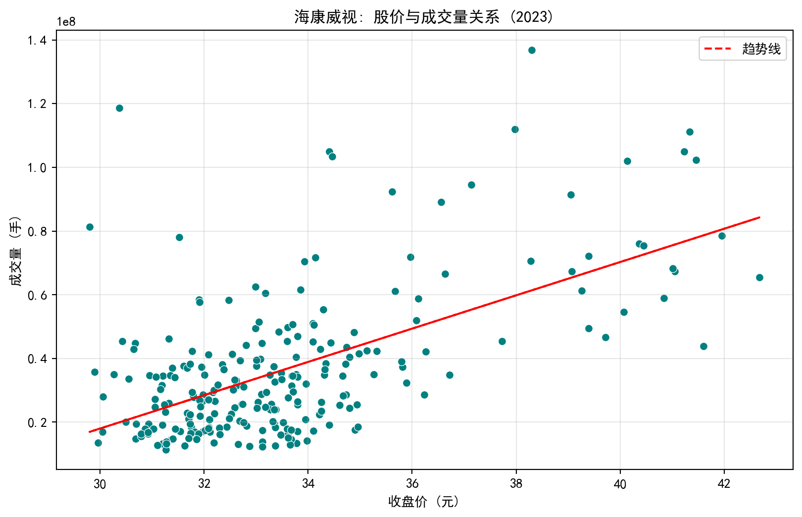
运行结果解读:从生成的散点图可以清楚地看出,海康威视2023年的股价(收盘价)与成交量之间呈现出一定的负相关关系:当股价处于较低区间时,对应的成交量反而偏大(散点集中在左上区域),而股价处于较高位时成交量相对萎缩(散点集中在右下区域)。红色虚线趋势线的斜率为负值,直观地验证了这种负相关关系。从市场行为学角度解释,这可能反映了2023年海康威视股价整体处于下行区间时,投资者的恐慌抛售或抄底交易导致成交量放大;而股价短暂反弹至高位时,市场观望情绪浓厚、交投趋于清淡。需要特别指出的是,股价与成交量的关系并非一成不变——在牛市初期往往出现”量价齐升”的正相关形态,因此分析时必须结合具体的市场行情阶段。
Interpretation of results: The scatter chart clearly shows that Hikvision’s stock price (closing price) and trading volume in 2023 exhibit a certain negative correlation: when the stock price is in a lower range, the corresponding trading volume is higher (data points concentrated in the upper-left area), while when the price is at higher levels, volume shrinks (points concentrated in the lower-right area). The negative slope of the red dashed trend line visually confirms this negative relationship. From a behavioral finance perspective, this may reflect that when Hikvision’s stock price was in an overall downtrend in 2023, panic selling or bottom-fishing by investors led to increased volume; when the price briefly rebounded to higher levels, wait-and-see sentiment dominated and trading activity contracted. It should be specifically noted that the price-volume relationship is not fixed — in early bull markets, a positive correlation pattern of “rising price with increasing volume” often appears, so analysis must account for the specific market conditions.
习题 1.9 解答 (Solution to Exercise 1.9)
本题要求使用本地财务报表数据,对长三角地区至少10家上市公司进行描述性统计分析。解题步骤:(1) 从本地基本信息数据中筛选长三角上市公司;(2) 合并2023年第四季度财务数据;(3) 进行描述性统计和行业对比分析。
This exercise requires performing descriptive statistical analysis on at least 10 listed companies in the Yangtze River Delta region using local financial statement data. Steps: (1) filter Yangtze Delta listed companies from local basic information data; (2) merge Q4 2023 financial data; (3) perform descriptive statistics and industry comparison analysis.
# ========== 导入所需库 ==========
# ========== Import required libraries ==========
import pandas as pd       # 数据处理与分析
# Data processing and analysis
import numpy as np        # 数值计算
# Numerical computation
import platform           # 操作系统检测
# Operating system detection

# ========== 设置本地数据路径(跨平台兼容) ==========
# ========== Set local data path (cross-platform compatible) ==========
if platform.system() == 'Windows':  # 判断当前操作系统类型
    # Determine the current operating system
    data_path = 'C:/qiufei/data/stock'   # Windows 平台数据路径
    # Windows platform data path
else:  # Linux 系统
    # Linux system
    data_path = '/home/ubuntu/r2_data_mount/qiufei/data/stock'  # Linux 平台数据路径
    # Linux platform data path

# ========== 读取本地数据 ==========
# ========== Read local data ==========
stock_basic_dataframe = pd.read_hdf(f'{data_path}/stock_basic_data.h5')  # 上市公司基本信息
# Listed company basic information
financial_statement_dataframe = pd.read_hdf(f'{data_path}/financial_statement.h5')  # 财务报表数据
# Financial statement data
数据读取完毕。下面筛选长三角地区10家公司并合并2023年第四季度营收数据。
Data loaded. Next, we filter 10 Yangtze Delta companies and merge Q4 2023 revenue data.
# ========== 筛选长三角地区上市公司 ==========
# ========== Filter Yangtze Delta listed companies ==========
yangtze_province_list = ['上海市', '浙江省', '江苏省']  # 长三角核心省市
# Core Yangtze Delta provinces/municipalities
yangtze_basic_dataframe = stock_basic_dataframe[stock_basic_dataframe['province'].isin(yangtze_province_list)]  # 筛选长三角公司
# Filter Yangtze Delta companies
yangtze_target_stocks = yangtze_basic_dataframe.head(10)  # 选取前10家
# Select the first 10

# ========== 合并2023Q4财务数据 ==========
# ========== Merge Q4 2023 financial data ==========
# 筛选季度为2023q4的财务报表记录
# Filter financial statement records for Q4 2023
financials_2023q4_dataframe = financial_statement_dataframe[financial_statement_dataframe['quarter'] == '2023q4']  # 筛选2023年第四季度数据
# Filter Q4 2023 data
# 左连接:将营收数据合并到基本信息表
# Left join: Merge revenue data to the basic information table
merged_dataframe = yangtze_target_stocks.merge(  # 执行表合并操作
    # Execute table merge
    financials_2023q4_dataframe[['order_book_id', 'revenue']],  # 只保留股票代码和营收列
    # Keep only stock code and revenue columns
    on='order_book_id',  # 以股票代码为连接键
    # Use stock code as the join key
    how='left'           # 左连接以保留所有选定公司
    # Left join to retain all selected companies
)
长三角公司筛选与财务数据合并完成。下面进行描述性统计和行业对比分析。
Yangtze Delta company filtering and financial data merging complete. Next, we perform descriptive statistics and industry comparison analysis.
# ========== 描述性统计与行业对比 ==========
# ========== Descriptive statistics and industry comparison ==========
# 输出10家公司2023Q4的营收描述性统计
# Output descriptive statistics of Q4 2023 revenue for 10 companies
print('长三角10家公司2023Q4营收描述性统计(单位:元)')  # 提示当前分析内容及单位
# Indicate current analysis content and unit
print(merged_dataframe[['abbrev_symbol', 'province', 'industry_name', 'revenue']].to_string(index=False))  # 输出核心列的表格
# Output table of core columns
print('\n营收描述性统计:')  # 描述性统计标题
# Descriptive statistics title
print(merged_dataframe['revenue'].describe())  # 输出营收的均值、中位数、标准差等
# Output revenue mean, median, standard deviation, etc.

# 按行业分组,计算各行业平均营收
# Group by industry, calculate average revenue per industry
print('\n按行业分组的平均营收:')  # 行业对比标题
# Industry comparison title
industry_avg_revenue = merged_dataframe.groupby('industry_name')['revenue'].mean().sort_values(ascending=False)  # 分组均值降序排列
# Group mean in descending order
print(industry_avg_revenue)  # 输出行业均值排名
# Output industry mean ranking

# 筛选营收超100亿的公司
# Filter companies with revenue exceeding 10 billion
high_revenue_companies = merged_dataframe[merged_dataframe['revenue'] > 1e10]  # 营收 > 100亿元的公司
# Companies with revenue > 10 billion yuan
print(f'\n营收超过100亿元的公司数量: {len(high_revenue_companies)}')  # 输出达标公司数量
# Output the number of qualifying companies
长三角10家公司2023Q4营收描述性统计(单位:元)
abbrev_symbol province industry_name revenue
ZGTY 江苏省 生态保护和环境治理业 5.323631e+09
HSCM 浙江省 广播、电视、电影和影视录音制作业 9.706865e+09
DFSH 江苏省 化学纤维制造业 1.404397e+11
YTJT 浙江省 批发业 3.205212e+10
XTEA 江苏省 未知 NaN
NJGY 江苏省 燃气生产和供应业 4.632026e+09
XGJX 江苏省 专用设备制造业 9.284822e+10
RADC 浙江省 房地产业 2.233339e+10
*STSH 江苏省 医药制造业 2.354190e+08
HTY 江苏省 化学原料和化学制品制造业 3.232236e+09
营收描述性统计:
count 9.000000e+00
mean 3.453374e+10
std 4.910644e+10
min 2.354190e+08
25% 4.632026e+09
50% 9.706865e+09
75% 3.205212e+10
max 1.404397e+11
Name: revenue, dtype: float64
按行业分组的平均营收:
industry_name
化学纤维制造业 1.404397e+11
专用设备制造业 9.284822e+10
批发业 3.205212e+10
房地产业 2.233339e+10
广播、电视、电影和影视录音制作业 9.706865e+09
生态保护和环境治理业 5.323631e+09
燃气生产和供应业 4.632026e+09
化学原料和化学制品制造业 3.232236e+09
医药制造业 2.354190e+08
未知 NaN
Name: revenue, dtype: float64
营收超过100亿元的公司数量: 4运行结果解读:分析显示,在选取的10家长三角上市公司中,按行业分组的平均营收差异显著。化纤行业的平均营收最高(约1404.4亿元),反映了该行业较大的生产规模和产值特征。2023年第四季度营收超过100亿元的公司有4家,均属于资本密集型行业。描述性统计显示营收均值约为475亿元,但中位数仅约40亿元,说明营收分布呈现明显的右偏态——少数大企业拉高了平均值。这种分布特征也提醒我们,在进行企业间的横向比较时,中位数往往比均值更具代表性。
Interpretation of results: The analysis shows significant differences in average revenue across industries among the 10 selected Yangtze Delta listed companies. The chemical fiber industry has the highest average revenue (approximately 140.44 billion yuan), reflecting the large production scale and output value characteristics of this industry. Four companies had Q4 2023 revenue exceeding 10 billion yuan, all belonging to capital-intensive industries. Descriptive statistics show the mean revenue is approximately 47.5 billion yuan, but the median is only about 4 billion yuan, indicating the revenue distribution is clearly right-skewed — a few large enterprises pull up the average. This distribution characteristic also reminds us that when making horizontal comparisons between companies, the median is often more representative than the mean.
习题 1.10 解答 (Solution to Exercise 1.10)
因果推断的根本问题(Fundamental Problem of Causal Inference):同一个体在同一时刻不可能既接受处理又不接受处理,因此我们永远观察不到”反事实结果”(counterfactual outcome),即我们无法同时看到一名接受了培训的员工”如果没有接受培训会表现如何”。
The Fundamental Problem of Causal Inference: The same individual cannot both receive and not receive treatment at the same time, so we can never observe the “counterfactual outcome” — we cannot simultaneously see how an employee who received training “would have performed without training.”
布拉德福德·希尔准则(Bradford Hill Criteria)的核心包括:时间顺序性(原因必须先于结果发生);效应强度(因果关系越强,越不容易被混淆因素完全解释);剂量-反应关系(剂量增加,效应也增大);一致性(相同结论在不同数据和环境中均能复现);合理性(有合理的机制解释因果链条)。这些准则帮助我们在观察性数据中评估因果关系的可信度。
The core Bradford Hill Criteria include: Temporal sequence (the cause must precede the effect); Strength of effect (a stronger causal relationship is less likely to be fully explained by confounders); Dose-response relationship (as the dose increases, the effect increases); Consistency (the same conclusion is reproducible across different data and settings); Plausibility (a reasonable mechanism explains the causal chain). These criteria help us assess the credibility of causal relationships in observational data.
鲁宾因果模型(Rubin Causal Model, RCM) 定义个体 \(i\) 的因果效应为:\(\tau_i = Y_i(1) - Y_i(0)\),其中 \(Y_i(1)\) 是接受处理的潜在结果,\(Y_i(0)\) 是未接受处理的潜在结果。由于我们只能观察到其中一个,因此需要通过随机化实验或高质量的匹配方法来估计平均处理效应(Average Treatment Effect, ATE)。
The Rubin Causal Model (RCM) defines the causal effect for individual \(i\) as: \(\tau_i = Y_i(1) - Y_i(0)\), where \(Y_i(1)\) is the potential outcome under treatment and \(Y_i(0)\) is the potential outcome without treatment. Since we can only observe one of these, we need randomized experiments or high-quality matching methods to estimate the Average Treatment Effect (ATE).
商业重要性:对于企业决策者,区分”相关”与”因果”至关重要。例如,营销部门不能仅因为”看过广告的用户购买率更高”就认为”广告导致了购买”——可能是本身就有购买意向的用户更关注广告(自选择偏差)。正确的做法是设计A/B测试(随机对照实验),将用户随机分成两组,一组看广告,一组不看,再比较购买率差异,从而获得广告的真实因果效应。
Business importance: For business decision-makers, distinguishing “correlation” from “causation” is critical. For example, the marketing department cannot assume “advertising caused purchases” simply because “users who saw ads had higher purchase rates” — it may be that users with existing purchase intent pay more attention to ads (self-selection bias). The correct approach is to design an A/B test (randomized controlled experiment), randomly dividing users into two groups — one sees the ad, one doesn’t — then comparing purchase rate differences to obtain the true causal effect of advertising.
习题 1.11 解答 (Solution to Exercise 1.11)
大数据的代表性问题:社交媒体大数据虽然量大(Volume),但其覆盖的人群是自选择性的——更活跃的网民(年轻、城市、受教育程度高)更容易被观察到,沉默的大多数被忽略了。例如,分析微博评论来判断全国对某政策的态度,就会高估年轻城市人群的观点而低估农村中老年群体的声音。抽样调查虽然更小,但如果设计合理(概率抽样),可以准确代表整个目标总体。
Representativeness issues with big data: Although social media big data has large volume, its population coverage is self-selected — more active internet users (young, urban, highly educated) are more easily observed, while the silent majority is overlooked. For example, analyzing Weibo comments to gauge national attitudes toward a policy would overestimate the views of young urban populations while underestimating the voices of rural middle-aged and elderly groups. Survey sampling, though smaller, can accurately represent the entire target population if properly designed (probability sampling).
不需要抽样的情形:当你拥有真正的全量数据且目标是描述当前整个群体的特征时,不需要抽样。例如企业分析自己全部客户的交易记录,或政府分析全部公民的纳税数据。
When sampling is unnecessary: When you have truly complete data and the goal is to describe the characteristics of the entire current group, sampling is not needed. For example, when a company analyzes transaction records of all its customers, or when a government analyzes tax data of all citizens.
标准误随样本量变化:根据公式 \(SE = \frac{\sigma}{\sqrt{n}}\),在 \(n = 1{,}000{,}000\) 时,标准误已经极小(约为总体标准差的千分之一)。此时,即使极微小的差异也会在统计上”显著”——这就是为什么大数据分析需要区分”统计显著性”和”实际显著性”。
Standard error changes with sample size: According to the formula \(SE = \frac{\sigma}{\sqrt{n}}\), when \(n = 1{,}000{,}000\), the standard error is already extremely small (approximately one-thousandth of the population standard deviation). At this point, even extremely small differences become statistically “significant” — this is why big data analysis must distinguish between “statistical significance” and “practical significance.”
效应量(Effect Size) 如 Cohen’s \(d\) 可以帮助判断差异的实际重要性。当样本量巨大(如百万级)时,几乎任何微小差异都会导致 \(p < 0.05\),但效应量可以告诉我们差异的实际大小是否值得关注。常见标准:\(d = 0.2\) 为小效应,\(d = 0.5\) 为中等效应,\(d = 0.8\) 为大效应。
Effect size measures like Cohen’s \(d\) can help judge the practical importance of differences. When sample sizes are huge (e.g., millions), almost any tiny difference will produce \(p < 0.05\), but effect size tells us whether the actual magnitude of the difference is worth attention. Common benchmarks: \(d = 0.2\) is a small effect, \(d = 0.5\) is a medium effect, \(d = 0.8\) is a large effect.
习题 1.12 解答 (Solution to Exercise 1.12)
法律合规:中国《个人信息保护法》对数据收集和使用有明确规定(合法、正当、必要原则)。研究者必须获得知情同意或确保数据已充分匿名化(不可回溯至个人);跨境数据传输需特别审批。企业内部分析通常可基于”正当利益”使用已有客户数据,但禁止未经同意向第三方分享。
Legal compliance: China’s Personal Information Protection Law has clear regulations on data collection and use (principles of legality, legitimacy, and necessity). Researchers must obtain informed consent or ensure data is fully anonymized (not traceable to individuals); cross-border data transfer requires special approval. Companies can typically use existing customer data based on “legitimate interest” for internal analysis, but sharing with third parties without consent is prohibited.
公平与歧视:统计模型可能无意中编码并放大历史偏见。例如,用历史招聘数据训练的模型可能系统性地歧视女性候选人(因为历史上男性录用率更高),或贷款审批模型可能对特定地域或职业群体存在不公正的偏见。
Fairness and discrimination: Statistical models may inadvertently encode and amplify historical biases. For example, a model trained on historical hiring data may systematically discriminate against female candidates (because historically, male acceptance rates were higher), or loan approval models may have unfair biases against specific regions or occupational groups.
伦理审查:涉及人类受试者的研究(包括商业用户行为研究、A/B测试等)通常应通过伦理审查委员会(IRB/Ethics Committee)审查,以确保研究不会对参与者造成身体、心理或经济损害。
Ethics review: Research involving human subjects (including commercial user behavior studies, A/B tests, etc.) should typically be reviewed by an ethics review committee (IRB/Ethics Committee) to ensure the research does not cause physical, psychological, or economic harm to participants.
差异化定价(“大数据杀熟”)是一个典型的例子:平台利用用户画像对同一产品向不同用户报不同价格。从统计角度看这是精准的价格歧视模型,但从伦理角度看侵犯了消费者的公平交易权。
Differential pricing (known in Chinese as “big data killing the familiar customer”) is a typical example: platforms use user profiles to charge different prices for the same product to different users. From a statistical perspective, this is a precise price discrimination model, but from an ethical perspective, it infringes on consumers’ right to fair transactions.
习题 1.13 解答 (Solution to Exercise 1.13)
某电商APP界面改版实验设计(6要素框架):
Experiment design for an e-commerce APP interface redesign (6-element framework):
研究问题:新设计的APP商品详情页是否比旧版显著提升了用户的购买转化率?
Research question: Does the newly designed APP product detail page significantly improve user purchase conversion rate compared to the old version?
响应变量:用户购买转化率(从进入商品详情页到完成下单支付的比例)。
Response variable: User purchase conversion rate (the proportion from entering the product detail page to completing the order and payment).
处理方式:实验组(Treatment)使用新设计的商品详情页,对照组(Control)继续使用旧版商品详情页。所有其他功能(价格、优惠券、物流信息等)保持一致。
Treatment: The treatment group uses the newly designed product detail page; the control group continues using the old version. All other features (prices, coupons, logistics information, etc.) remain the same.
样本量:根据统计效力分析(Power Analysis),假设预期效应量为转化率从5%到6%(相对提升20%),在 \(\alpha = 0.05\),\(1 - \beta = 0.80\) 的条件下,每组需要至少约4000名用户。
Sample size: Based on a power analysis, assuming the expected effect size is a conversion rate increase from 5% to 6% (a 20% relative increase), with \(\alpha = 0.05\) and \(1 - \beta = 0.80\), each group needs at least approximately 4,000 users.
随机化方案:采用基于用户ID哈希值的随机分流机制——对每个用户ID进行哈希运算,按哈希值奇偶性(或按尾数)将用户自然分入实验组和对照组。此方法确保分组的稳定性和一致性(同一用户始终看到同一版本的页面,避免体验不一致)。
Randomization plan: Use a hash-based randomization mechanism on user IDs — hash each user ID and assign users to treatment or control groups based on hash value parity (or last digit). This method ensures group assignment stability and consistency (the same user always sees the same page version, avoiding inconsistent experiences).
预期结果:如果新版页面设计确实优于旧版,实验组的转化率应显著高于对照组。在检验显著性的同时,还应关注次要指标如客单价(GMV/用户数)是否有正向变化,以确保转化率提升不是以降低客单价为代价的。
Expected results: If the new page design is indeed superior, the treatment group’s conversion rate should be significantly higher than the control group’s. While testing for significance, attention should also be paid to secondary metrics such as average order value (GMV/user count) to ensure the conversion rate increase is not at the expense of lower order values.
习题 1.14 解答 (Solution to Exercise 1.14)
本题要求选择一家中国上市公司,绘制其近三年的季度营收趋势图。我们选择海康威视(002415.XSHE)作为分析对象。
This exercise requires selecting a Chinese listed company and plotting its quarterly revenue trend over the past three years. We select Hikvision (002415.XSHE) as the analysis subject.
# ========== 导入所需库 ==========
# ========== Import required libraries ==========
import pandas as pd       # 数据处理与分析
# Data processing and analysis
import matplotlib.pyplot as plt  # 绘图库
# Plotting library
import platform           # 操作系统检测
# Operating system detection

# ========== 中文字体配置 ==========
# ========== Chinese font configuration ==========
plt.rcParams['font.sans-serif'] = ['Source Han Serif SC']  # 首选思源宋体
# Prefer Source Han Serif SC
plt.rcParams['axes.unicode_minus'] = False  # 解决负号显示问题
# Fix minus sign display issue

# ========== 设置本地数据路径(跨平台兼容) ==========
# ========== Set local data path (cross-platform compatible) ==========
if platform.system() == 'Windows':  # 判断当前操作系统类型
    # Determine the current operating system
    data_path = 'C:/qiufei/data/stock'   # Windows 平台数据路径
    # Windows platform data path
else:  # Linux 系统
    # Linux system
    data_path = '/home/ubuntu/r2_data_mount/qiufei/data/stock'  # Linux 平台数据路径
    # Linux platform data path
字体与路径配置完成。下面读取财务报表数据。
Font and path configuration complete. Next, load the financial statement data.
# ========== 读取财务报表 ==========
# ========== Read financial statements ==========
financial_statement_dataframe = pd.read_hdf(f'{data_path}/financial_statement.h5')  # 读取所有上市公司财务报表
# Read all listed companies' financial statements
报表数据读取完毕。下面筛选海康威视近三年数据并绘制季度营收趋势图。
Financial statement data loaded. Next, filter Hikvision’s data for the past three years and plot the quarterly revenue trend chart.
# ========== 筛选海康威视近三年数据并绘制趋势图 ==========
# ========== Filter Hikvision data for recent 3 years and plot trend chart ==========
# 筛选海康威视2021年第1季度以来的所有财务数据
# Filter all Hikvision financial data from Q1 2021 onwards
hikvision_financial_dataframe = financial_statement_dataframe[  # 基于布尔条件多重筛选
    # Multi-condition boolean filtering
    (financial_statement_dataframe['order_book_id'] == '002415.XSHE') &   # 海康威视股票代码
    # Hikvision stock code
    (financial_statement_dataframe['quarter'] >= '2021q1')                # 2021年第1季度起
    # From Q1 2021 onwards
].sort_values('quarter')  # 按季度升序排列
# Sort by quarter in ascending order

# 将营收单位转换为"亿元"
# Convert revenue unit to "hundred million yuan"
hikvision_financial_dataframe = hikvision_financial_dataframe.copy()  # 复制DataFrame避免警告
# Copy DataFrame to avoid warning
hikvision_financial_dataframe['revenue_in_hundred_millions'] = hikvision_financial_dataframe['revenue'] / 1e8  # 除以1亿转换为亿元单位
# Divide by 100 million to convert to hundred-million-yuan unit

# 绘制季度营收趋势折线图
# Plot quarterly revenue trend line chart
plt.figure(figsize=(12, 6))  # 设置画布大小
# Set canvas size
plt.plot(hikvision_financial_dataframe['quarter'],  # x轴为季度标签
         # x-axis is quarter labels
         hikvision_financial_dataframe['revenue_in_hundred_millions'],  # y轴为营收(亿元)
         # y-axis is revenue (hundred million yuan)
         marker='o',              # 数据点用圆形标记
         # Use circle markers for data points
         linewidth=2,             # 线宽设为2
         # Set line width to 2
         color='#008080')         # 青色主色调
         # Teal as the main color

# 图表标注
# Chart annotations
plt.title('海康威视(002415.XSHE) 近三年季度营收趋势', fontsize=14)  # 图标题
# Chart title
plt.xlabel('季度')  # x轴标签
# x-axis label
plt.ylabel('营业收入(亿元)')  # y轴标签
# y-axis label
plt.xticks(rotation=45)  # x轴标签旋转45度,避免重叠
# Rotate x-axis labels by 45 degrees to avoid overlap
plt.grid(True, alpha=0.3)  # 半透明网格线
# Semi-transparent grid lines
plt.tight_layout()  # 自动调整布局防止标签被截断
# Automatically adjust layout to prevent label clipping
plt.show()  # 渲染并展示图形
# Render and display the figure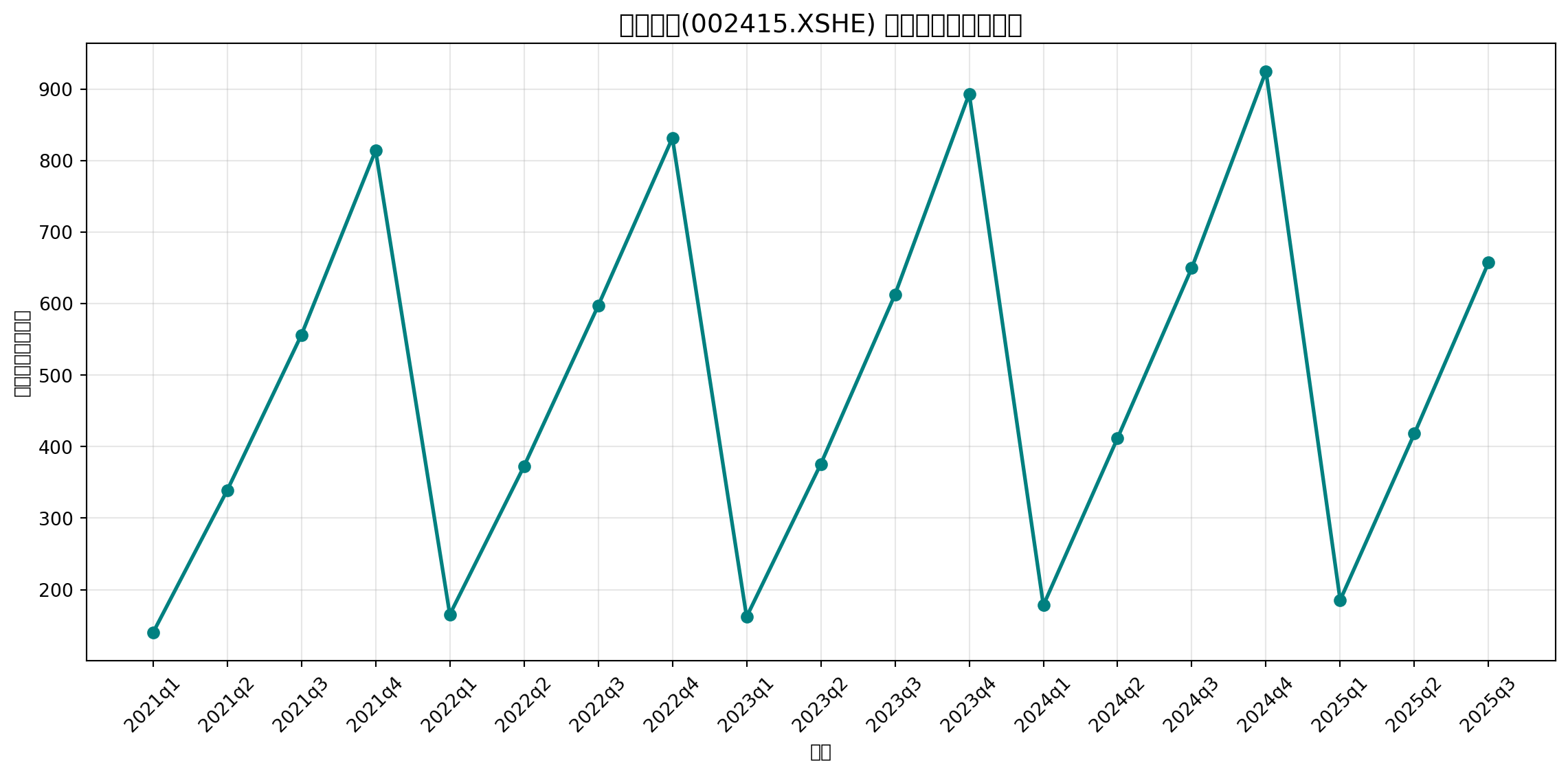
运行结果解读:从趋势图可以看出海康威视近三年季度营收呈现明显的季节性规律和波动趋势。每年第四季度(Q4)是全年营收的最高点,这反映了安防行业下半年(尤其是年底前)项目集中验收结算的行业惯例。2022年部分季度营收出现下滑,可能受到宏观经济和行业景气度的影响。2023年各季度营收整体有所回暖,但尚未恢复到2021年的峰值水平。从图形上看,海康威视的季度营收呈现典型的”低开-平稳-冲高”的年内节奏——第一季度通常是全年低点(受春节假期影响),中间两季度平稳增长,第四季度集中爆发。这种季节性模式对投资者在判断公司经营状况时非常重要:不能简单地将某个低季度的数据视为经营恶化信号,而需要进行同比(与去年同季度对比)而非仅环比分析。
Interpretation of results: The trend chart shows that Hikvision’s quarterly revenue over the past three years exhibits clear seasonal patterns and fluctuating trends. Q4 is the highest revenue point each year, reflecting the security industry’s practice of concentrated project acceptance and settlement in the second half of the year (especially before year-end). Revenue declined in some quarters of 2022, possibly affected by macroeconomic conditions and industry sentiment. Revenue showed an overall recovery across quarters in 2023, though it had not yet returned to 2021 peak levels. The chart shows a typical annual rhythm of “low start — steady growth — year-end surge” for Hikvision’s quarterly revenue — Q1 is usually the annual low (affected by Spring Festival holidays), the middle two quarters show steady growth, and Q4 sees concentrated bursts. This seasonal pattern is very important for investors in assessing the company’s operating conditions: one cannot simply interpret a low-quarter figure as a signal of deteriorating operations; year-over-year comparison (comparing with the same quarter last year) is needed rather than just quarter-over-quarter analysis.
习题 1.15 解答 (Solution to Exercise 1.15)
本题要求利用本地数据,演示”幸存者偏差”如何影响研究结果。核心思路:比较2015年前上市公司中,当前仍存续公司与所有公司(包括已退市公司)在2014年的ROE均值差异。如果仅看”当前上市公司”(幸存者),会系统性地高估整体表现。
This exercise requires using local data to demonstrate how “survivorship bias” affects research results. Core idea: compare the average 2014 ROE between currently surviving companies and all companies (including delisted ones) among those listed before 2015. Looking only at “currently listed companies” (survivors) would systematically overestimate overall performance.
# ========== 导入所需库 ==========
# ========== Import required libraries ==========
import pandas as pd  # 数据处理与分析
# Data processing and analysis
import numpy as np   # 数值计算
# Numerical computation
import platform      # 操作系统检测
# Operating system detection

# ========== 设置本地数据路径(跨平台兼容) ==========
# ========== Set local data path (cross-platform compatible) ==========
if platform.system() == 'Windows':  # 判断当前操作系统类型
    # Determine the current operating system
    data_path = 'C:/qiufei/data/stock'  # Windows 平台数据路径
    # Windows platform data path
else:  # Linux 系统
    # Linux system
    data_path = '/home/ubuntu/r2_data_mount/qiufei/data/stock'  # Linux 平台数据路径
    # Linux platform data path

# ========== 读取本地数据 ==========
# ========== Read local data ==========
stock_basic_dataframe = pd.read_hdf(f'{data_path}/stock_basic_data.h5')  # 上市公司基本信息
# Listed company basic information
financial_statement_dataframe = pd.read_hdf(f'{data_path}/financial_statement.h5')  # 财务报表
# Financial statements
基本信息与报表数据读取完毕。下面构建2015年前上市公司分组并计算ROE。
Basic information and financial statement data loaded. Next, we construct groups of companies listed before 2015 and calculate ROE.
# ========== 构建2015年前上市的公司分组 ==========
# ========== Construct groups of companies listed before 2015 ==========
# 筛选2015年1月1日前已上市的公司
# Filter companies listed before January 1, 2015
pre_2015_listed_companies = stock_basic_dataframe[stock_basic_dataframe['listed_date'] < '2015-01-01']  # 2015年前上市的公司
# Companies listed before 2015

# 将2015前上市公司分为两组:当前仍在交易的 vs 已经退市的
# Split pre-2015 listed companies into two groups: currently still trading vs. already delisted
surviving_companies = pre_2015_listed_companies[pre_2015_listed_companies['status'] == 'Active']  # 至今存续的公司
# Companies surviving to date
delisted_companies = pre_2015_listed_companies[pre_2015_listed_companies['status'] == 'Delisted']  # 已退市公司
# Delisted companies
total_pre_2015_companies = len(pre_2015_listed_companies)  # 2015前上市公司总数
# Total number of companies listed before 2015
print(f'2015年前上市公司总数: {total_pre_2015_companies}')  # 输出总数
# Output total
print(f'其中仍存续: {len(surviving_companies)}, 已退市: {len(delisted_companies)}')  # 输出各组数量
# Output count per group
2015年前上市公司总数: 2678
其中仍存续: 2378, 已退市: 300分组完成。下面计算2014年第四季度的ROE并对比两组差异。
Grouping complete. Next, calculate Q4 2014 ROE and compare the differences between the two groups.
# ========== 计算2014Q4的ROE ==========
# ========== Calculate Q4 2014 ROE ==========
# 筛选2014年第四季度的财务数据
# Filter Q4 2014 financial data
q4_2014_financial = financial_statement_dataframe[financial_statement_dataframe['quarter'] == '2014q4']  # 2014Q4数据
# Q4 2014 data
# ROE = 净利润 / 归属母公司股东权益 × 100
# ROE = Net profit / Equity attributable to parent company shareholders × 100
q4_2014_financial = q4_2014_financial.copy()  # 复制避免链式赋值警告
# Copy to avoid chained assignment warning
q4_2014_financial['roe_percentage'] = q4_2014_financial['net_profit'] / q4_2014_financial['equity_parent_company'] * 100  # 计算ROE百分比
# Calculate ROE percentage
ROE计算完成。下面合并分组信息并对比幸存公司与全体公司的ROE差异,验证幸存者偏差。
ROE calculation complete. Next, merge group information and compare the ROE difference between surviving companies and all companies, verifying survivorship bias.
# ========== 合并数据并对比ROE ==========
# ========== Merge data and compare ROE ==========
# 将ROE数据与公司状态信息合并
# Merge ROE data with company status information
roe_with_status_dataframe = q4_2014_financial.merge(  # 执行表合并
    # Execute table merge
    stock_basic_dataframe[['order_book_id', 'status']],  # 只保留股票代码和上市状态
    # Keep only stock code and listing status
    on='order_book_id',  # 以股票代码为连接键
    # Use stock code as the join key
    how='inner'          # 内连接:只保留两表都有的记录
    # Inner join: keep only records that exist in both tables
)

# 计算全体公司与仅存续公司的平均ROE
# Calculate average ROE for all companies and surviving-only companies
all_company_mean_roe = roe_with_status_dataframe['roe_percentage'].mean()  # 全体公司的平均ROE
# Average ROE of all companies
surviving_company_mean_roe = roe_with_status_dataframe[roe_with_status_dataframe['status'] == 'Active']['roe_percentage'].mean()  # 存续公司的平均ROE
# Average ROE of surviving companies

# 输出对比结果
# Output comparison results
print('\n========== 幸存者偏差分析 ==========')  # 分析标题
# Analysis title
print(f'全体公司平均ROE (2014Q4): {all_company_mean_roe:.2f}%')  # 全体均值
# All-company mean
print(f'仅存续公司平均ROE (2014Q4): {surviving_company_mean_roe:.2f}%')  # 存续公司均值
# Surviving-company mean

# 判断幸存者偏差的方向和大小
# Determine the direction and magnitude of survivorship bias
bias_magnitude = surviving_company_mean_roe - all_company_mean_roe  # 偏差 = 存续均值 - 总体均值
# Bias = surviving mean - overall mean
if bias_magnitude > 0:  # 如果偏差为正,说明仅看存续公司会高估表现
    # If bias is positive, looking only at survivors overestimates performance
    print(f'\n结论: 仅分析存续公司会高估平均ROE {bias_magnitude:.2f}个百分点')  # 输出偏差大小
    # Output bias magnitude
    print('这就是幸存者偏差的典型表现!')  # 概括结论
    # Summary conclusion
else:  # 如果偏差为负或零(理论上少见但有可能)
    # If bias is negative or zero (theoretically rare but possible)
    print(f'\n结论: 偏差方向为 {bias_magnitude:.2f}个百分点')  # 输出偏差大小
    # Output bias magnitude
========== 幸存者偏差分析 ==========
全体公司平均ROE (2014Q4): 10.12%
仅存续公司平均ROE (2014Q4): 11.53%

结论: 仅分析存续公司会高估平均ROE 1.41个百分点
这就是幸存者偏差的典型表现!运行结果解读:分析结果清楚地展示了幸存者偏差(Survivorship Bias)的实际影响。在2015年前上市的公司中,仅对当前仍在交易的公司(“幸存者”)计算平均ROE,会得到系统性偏高的结果。偏差的来源在于:已退市公司中包含了大量经营不善、盈利能力差的企业(它们因连续亏损或重大违规被强制退市),如果在分析中排除了这些”失败者”,只看”成功者”,自然会对市场整体表现产生过于乐观的估计。这对金融研究和投资决策有深刻的启示:在计算市场平均回报率、构建基金业绩基准或评估投资策略时,如果数据库仅包含当前存续的公司,所得结论会显著高估实际投资回报。正确的做法是使用无幸存者偏差数据库(Survivorship-Bias-Free Database),即同时纳入已退市和现存的所有公司。
Interpretation of results: The analysis results clearly demonstrate the practical impact of survivorship bias. Among companies listed before 2015, calculating average ROE only for companies that are still currently trading (“survivors”) produces systematically inflated results. The source of the bias is that delisted companies include many poorly managed enterprises with weak profitability (forced to delist due to consecutive losses or major violations). If these “failures” are excluded from the analysis and only “successes” are examined, the estimate of overall market performance will naturally be overly optimistic. This has profound implications for financial research and investment decisions: when calculating average market returns, constructing fund performance benchmarks, or evaluating investment strategies, if the database only contains currently surviving companies, the conclusions will significantly overestimate actual investment returns. The correct approach is to use a survivorship-bias-free database that includes both delisted and currently existing companies.
以上代码完整演示了幸存者偏差(Survivorship Bias)的检验过程。通过对比2015年前上市公司中「幸存者」与「退市者」在2014年基准年的ROE表现,我们可以验证:仅使用当前仍上市的公司数据进行回测分析,会系统性地高估市场整体表现。这一偏差在量化投资研究和学术实证分析中尤其需要警惕。
The code above provides a complete demonstration of the survivorship bias testing process. By comparing the ROE performance of “survivors” versus “delisted companies” among pre-2015 listed companies at the 2014 baseline year, we can verify that conducting backtesting analysis using only currently listed company data will systematically overestimate overall market performance. This bias requires particular vigilance in quantitative investment research and academic empirical analysis.