# ========== 导入所需库 ==========
# ========== Import required libraries ==========
import pandas as pd                    # 数据处理库
# Data manipulation library
import numpy as np                     # 数值计算库
# Numerical computation library
from sklearn.tree import DecisionTreeClassifier, plot_tree, export_text  # 决策树分类器及可视化工具
# Decision tree classifier and visualization tools
from sklearn.model_selection import train_test_split, cross_val_score    # 数据拆分与交叉验证
# Data splitting and cross-validation
from sklearn.metrics import accuracy_score, classification_report, roc_auc_score, roc_curve  # 评估指标
# Evaluation metrics
import matplotlib.pyplot as plt        # 数据可视化库
# Data visualization library
import platform                        # 平台检测模块
# Platform detection module

# ========== 中文字体设置 ==========
# ========== Chinese font configuration ==========
if platform.system() == 'Linux':       # Linux系统
    # Linux system
    plt.rcParams['font.sans-serif'] = ['Source Han Serif SC', 'SimHei', 'DejaVu Sans']  # 思源宋体优先
    # Source Han Serif SC preferred
else:                                  # Windows系统
    # Windows system
    plt.rcParams['font.sans-serif'] = ['SimHei', 'Microsoft YaHei']  # 黑体优先
    # SimHei preferred
plt.rcParams['axes.unicode_minus'] = False  # 解决负号显示问题
# Fix minus sign display issue

# ========== 第1步:读取本地财务数据 ==========
# ========== Step 1: Load local financial data ==========
if platform.system() == 'Linux':       # 根据操作系统选择数据路径
    # Select data path based on operating system
    data_path = '/home/ubuntu/r2_data_mount/qiufei/data/stock'  # Linux路径
    # Linux path
else:                                                          # 否则为Windows系统
    # Otherwise Windows system
    data_path = 'C:/qiufei/data/stock'                          # Windows路径
    # Windows path

financial_statement_dataframe = pd.read_hdf(f'{data_path}/financial_statement.h5')  # 读取财务报表
# Read financial statements
stock_basic_info_dataframe = pd.read_hdf(f'{data_path}/stock_basic_data.h5')        # 读取股票基本信息
# Read stock basic information12 基于树的机器学习方法 (Tree-Based Machine Learning Methods)
决策树及其集成方法(随机森林、梯度提升)是现代机器学习中最强大的预测工具之一,在商业分析、金融风控、信用评级等领域有广泛应用。树方法能自动捕捉非线性关系和变量交互效应,无需显式指定模型形式,且对异常值和缺失数据具有天然的稳健性。本章首先介绍决策树的基本算法(小节 12.2),然后讨论随机森林(小节 12.4)和XGBoost(小节 12.5)等集成方法,最后探讨模型可解释性(小节 12.6)。
Decision trees and their ensemble methods (random forests, gradient boosting) are among the most powerful predictive tools in modern machine learning, with broad applications in business analytics, financial risk management, and credit rating. Tree-based methods can automatically capture nonlinear relationships and variable interaction effects without explicitly specifying the model form, and are naturally robust to outliers and missing data. This chapter first introduces the basic decision tree algorithm (小节 12.2), then discusses ensemble methods such as random forests (小节 12.4) and XGBoost (小节 12.5), and finally explores model interpretability (小节 12.6).
12.1 树方法在量化金融中的典型应用 (Typical Applications of Tree Methods in Quantitative Finance)
决策树及其集成方法打破了传统统计建模对线性假设和参数形式的依赖,在金融领域展现出强大的预测能力。以下展示其在中国资本市场中的核心应用场景。
Decision trees and their ensemble methods break free from the dependence on linearity assumptions and parametric forms in traditional statistical modeling, demonstrating strong predictive power in the financial domain. The following presents their core application scenarios in the Chinese capital market.
12.1.1 应用一:基于机器学习的量化选股 (Application 1: Machine Learning-Based Quantitative Stock Selection)
传统多因子选股模型(参见 章节 10)假设因子与收益率之间存在线性关系。但A股市场中,因子与收益率的关系往往是非线性的且存在大量交互效应。随机森林和XGBoost等集成树方法可以自动捕捉这些复杂关系。利用 valuation_factors_quarterly_15_years.h5 中的估值因子作为特征,以下期股票收益率排名作为目标变量,可以构建预测能力显著优于线性模型的选股策略。
Traditional multi-factor stock selection models (see 章节 10) assume a linear relationship between factors and returns. However, in the A-share market, the relationship between factors and returns is often nonlinear with extensive interaction effects. Ensemble tree methods such as random forests and XGBoost can automatically capture these complex relationships. Using valuation factors from valuation_factors_quarterly_15_years.h5 as features and next-period stock return rankings as the target variable, one can construct stock selection strategies with predictive power significantly superior to linear models.
12.1.2 应用二:信用评级与风险预警 (Application 2: Credit Rating and Risk Early Warning)
在信用风险评估中(参见 章节 11 中的Logistic回归方法),梯度提升树(XGBoost/LightGBM)因其卓越的预测精度已成为业界标准工具。基于 financial_statement.h5 中的财务指标(如流动比率、资产负债率、现金流比率等),树方法不仅能识别出关键风险因子,还能通过特征重要性(Feature Importance)和SHAP值提供可解释的风险归因分析。
In credit risk assessment (see the Logistic regression method in 章节 11), gradient boosting trees (XGBoost/LightGBM) have become the industry standard tool due to their outstanding predictive accuracy. Based on financial indicators from financial_statement.h5 (such as current ratio, debt-to-asset ratio, cash flow ratio, etc.), tree methods can not only identify key risk factors but also provide interpretable risk attribution analysis through Feature Importance and SHAP values.
12.1.3 应用三:市场状态识别与择时策略 (Application 3: Market Regime Identification and Timing Strategies)
将 stock_price_pre_adjusted.h5 中的技术指标(如波动率、成交量变化、均线偏离度等)作为特征,以未来市场涨跌作为目标变量,可以训练树模型识别不同的市场状态(牛市/熊市/震荡市),为投资择时提供参考。
Using technical indicators from stock_price_pre_adjusted.h5 (such as volatility, trading volume changes, moving average deviations, etc.) as features and future market movements as the target variable, tree models can be trained to identify different market regimes (bull/bear/sideways markets), providing references for investment timing decisions.
直观几何解释:
Intuitive Geometric Interpretation:
决策树本质上是用超矩形(Hyper-rectangles)来切割特征空间。
Decision trees essentially partition the feature space using hyper-rectangles.
每一刀(分割)都必须平行于坐标轴(\(X_j \leq s\))。
最终,特征空间被切成无数个不重叠的小方块(叶节点)。
相比于线性回归(用超平面切割),决策树能逼近任意形状的非线性边界,只要切得足够细(树足够深)。
Each cut (split) must be parallel to a coordinate axis (\(X_j \leq s\)).
Ultimately, the feature space is partitioned into numerous non-overlapping small rectangles (leaf nodes).
Compared to linear regression (which cuts with hyperplanes), decision trees can approximate nonlinear boundaries of arbitrary shapes, as long as the cuts are fine enough (the tree is deep enough).
但这也带来了过拟合的风险——切得太细,就变成了死记硬背。
However, this also introduces the risk of overfitting—cutting too finely amounts to memorizing the training data.
12.2 决策树算法 (Decision Tree Algorithms)
12.2.1 CART算法框架 (CART Algorithm Framework)
CART(Classification and Regression Trees)是最常用的决策树算法,采用贪心策略进行二叉递归分割。
CART (Classification and Regression Trees) is the most commonly used decision tree algorithm, employing a greedy strategy for binary recursive partitioning.
算法流程:
Algorithm Procedure:
初始化: 全部数据构成根节点
最优分割: 对当前节点,遍历所有特征\(j\)和所有可能的分割点\(s\):
- 定义两个区域:\(R_1(j,s) = \{X|X_j \leq s\}\),\(R_2(j,s) = \{X|X_j > s\}\)
- 选择使某种不纯度度量最小化的\((j^*, s^*)\)
递归分割: 对生成的两个子节点重复步骤2
停止条件: 节点样本数小于阈值,或不纯度不再下降,或达到最大深度
剪枝: 通过交叉验证选择最优复杂度参数
Initialization: All data forms the root node
Optimal Split: For the current node, iterate over all features \(j\) and all possible split points \(s\):
- Define two regions: \(R_1(j,s) = \{X|X_j \leq s\}\), \(R_2(j,s) = \{X|X_j > s\}\)
- Select \((j^*, s^*)\) that minimizes a certain impurity measure
Recursive Splitting: Repeat step 2 for each generated child node
Stopping Criteria: Node sample size falls below a threshold, impurity no longer decreases, or maximum depth is reached
Pruning: Select the optimal complexity parameter via cross-validation
12.2.2 分类树的分割准则 (Splitting Criteria for Classification Trees)
对于分类问题,常用的不纯度度量包括:
For classification problems, commonly used impurity measures include:
1. 基尼不纯度(Gini Impurity)
1. Gini Impurity
\[ G(p) = \sum_{k=1}^K p_k(1-p_k) = 1 - \sum_{k=1}^K p_k^2 \tag{12.1}\]
式 12.1 中,\(p_k\)是节点中第\(k\)类的样本比例。
In 式 12.1, \(p_k\) is the proportion of samples belonging to class \(k\) in the node.
基尼不纯度与熵的数学关系(泰勒展开)
Mathematical Relationship Between Gini Impurity and Entropy (Taylor Expansion)
为什么 CART 用 Gini 而 C4.5 用 Entropy?
Why does CART use Gini while C4.5 uses Entropy?
熵的定义:\(H(p) = -p \ln(p) - (1-p) \ln(1-p)\)
The definition of entropy: \(H(p) = -p \ln(p) - (1-p) \ln(1-p)\)
在 \(p=1\) 附近对 \(H(p)\) 进行一阶泰勒展开(\(\ln(x) \approx x-1\)):
Performing a first-order Taylor expansion of \(H(p)\) near \(p=1\) (\(\ln(x) \approx x-1\)):
\[ -\ln(p) \approx 1-p \]
代入熵公式:
Substituting into the entropy formula:
\[ H(p) \approx p(1-p) + (1-p)p = 2p(1-p) = G(p) \]
这说明:基尼不纯度实际上是熵的一阶近似。
This shows that: Gini impurity is actually a first-order approximation of entropy.
计算上:Gini不需要算对数,速度更快(在计算机算力稀缺的80年代很重要)。
性质上:两者极其相似,但在极端情况(极纯或极不纯)下略有差异。
Computationally: Gini does not require logarithm calculations and is faster (which was important in the 1980s when computing power was scarce).
In terms of properties: The two are extremely similar, but differ slightly in extreme cases (very pure or very impure).
2. 熵(Entropy)/信息增益
2. Entropy / Information Gain
什么是熵?
What is Entropy?
熵(Entropy) 是信息论中衡量不确定性或混乱程度的核心指标,由香农(Claude Shannon)在1948年提出。直观理解:如果一个事件的结果越难预测,它的熵就越高。
Entropy is the core metric in information theory for measuring uncertainty or disorder, proposed by Claude Shannon in 1948. Intuitively: the harder it is to predict the outcome of an event, the higher its entropy.
用一个简单例子来说明:
A simple example illustrates this:
一枚公平硬币(正面概率50%,反面概率50%):抛一次,你完全无法预测结果——不确定性最大,熵最高。
一枚灌铅硬币(正面概率99%,反面概率1%):抛一次,你几乎可以确定是正面——不确定性很低,熵很低。
一枚双面相同的硬币(正面概率100%):结果完全确定,没有任何不确定性——熵为零。
A fair coin (50% heads, 50% tails): flip it once, and you cannot predict the result at all—uncertainty is maximized, entropy is highest.
A loaded coin (99% heads, 1% tails): flip it once, and you can almost certainly predict heads—uncertainty is very low, entropy is very low.
A double-headed coin (100% heads): the result is completely certain, with no uncertainty—entropy is zero.
在决策树的语境中,我们用熵来衡量一个节点中样本标签的”混乱程度”:如果一个节点中所有样本都属于同一类别(纯净),熵为0;如果样本在各类别中均匀分布(完全混合),熵达到最大值。决策树的目标就是通过不断分裂,使子节点的熵尽可能低——即让每个叶节点尽可能”纯净”。
In the context of decision trees, we use entropy to measure the “disorder” of sample labels within a node: if all samples in a node belong to the same class (pure), entropy is 0; if samples are uniformly distributed across classes (completely mixed), entropy reaches its maximum. The goal of a decision tree is to reduce child node entropy as much as possible through successive splits—that is, to make each leaf node as “pure” as possible.
熵的数学公式如 式 12.2 所示:
The mathematical formula for entropy is shown in 式 12.2:
\[ H(p) = -\sum_{k=1}^K p_k \log_2 p_k \tag{12.2}\]
熵的公式如 式 12.2 所示。信息增益(Information Gain)定义为父节点熵与子节点加权平均熵的差(见 式 12.3):
The entropy formula is shown in 式 12.2. Information Gain is defined as the difference between the parent node entropy and the weighted average entropy of the child nodes (see 式 12.3):
\[ IG = H(\text{parent}) - \sum_{c \in \{L,R\}} \frac{n_c}{n} H(c) \tag{12.3}\]
3. 两种准则的比较
3. Comparison of the Two Criteria
| 准则 | 计算复杂度 | 特点 |
|---|---|---|
| Gini | 较低(无对数) | CART默认,偏好较大分区 |
| Entropy | 较高 | ID3/C4.5使用,更敏感于类别分布 |
| Criterion | Computational Complexity | Characteristics |
|---|---|---|
| Gini | Lower (no logarithm) | CART default, prefers larger partitions |
| Entropy | Higher | Used by ID3/C4.5, more sensitive to class distribution |
实践中,两者性能通常相近。
In practice, the performance of the two is generally similar.
12.2.3 回归树的分割准则 (Splitting Criteria for Regression Trees)
对于回归问题,使用均方误差(MSE)作为分割准则:
For regression problems, Mean Squared Error (MSE) is used as the splitting criterion:
\[ MSE = \frac{1}{n}\sum_{i=1}^n (y_i - \bar{y})^2 \tag{12.4}\]
如 式 12.4 所示。选择使两个子区域MSE加权之和最小的分割(见 式 12.5):
As shown in 式 12.4. The split that minimizes the weighted sum of MSE of the two child regions is selected (see 式 12.5):
\[ \min_{j,s} \left[ \frac{n_L}{n} MSE(R_L) + \frac{n_R}{n} MSE(R_R) \right] \tag{12.5}\]
其中\(n_L, n_R\)分别是左右子节点的样本数。
where \(n_L, n_R\) are the number of samples in the left and right child nodes, respectively.
12.2.4 最优分割点的搜索 (Search for the Optimal Split Point)
分割点搜索算法
Split Point Search Algorithm
对于特征\(X_j\):
For feature \(X_j\):
将\(n\)个样本按\(X_j\)值排序:\(x_{(1)j} \leq x_{(2)j} \leq ... \leq x_{(n)j}\)
候选分割点:\(\{s_i = \frac{x_{(i)j} + x_{(i+1)j}}{2}\}_{i=1}^{n-1}\)
对每个\(s_i\)计算不纯度减少量
选择不纯度减少最大的分割点
Sort the \(n\) samples by \(X_j\) values: \(x_{(1)j} \leq x_{(2)j} \leq ... \leq x_{(n)j}\)
Candidate split points: \(\{s_i = \frac{x_{(i)j} + x_{(i+1)j}}{2}\}_{i=1}^{n-1}\)
Compute the impurity reduction for each \(s_i\)
Select the split point with the greatest impurity reduction
计算复杂度: 对于\(p\)个特征,\(n\)个样本,每次分割需要\(O(np\log n)\)时间。
Computational Complexity: For \(p\) features and \(n\) samples, each split requires \(O(np\log n)\) time.
12.2.5 剪枝策略 (Pruning Strategies)
过拟合问题: 完全生长的树往往过拟合训练数据。
Overfitting Problem: A fully grown tree tends to overfit the training data.
代价复杂度剪枝(Cost-Complexity Pruning):
Cost-Complexity Pruning:
最小化:
Minimize:
\[ C_\alpha(T) = \sum_{m=1}^{|T|} \sum_{x_i \in R_m} L(y_i, c_m) + \alpha|T| \tag{12.6}\]
式 12.6 中各项含义如下:
The terms in 式 12.6 are defined as follows:
\(|T|\): 叶节点数(树的复杂度)
\(\alpha\): 复杂度参数(控制正则化强度)
通过交叉验证选择最优\(\alpha\)
\(|T|\): Number of leaf nodes (tree complexity)
\(\alpha\): Complexity parameter (controls regularization strength)
The optimal \(\alpha\) is selected via cross-validation
12.3 案例:上市公司违约风险预测 (Case Study: Default Risk Prediction for Listed Companies)
什么是基于决策树的信用风险评估?
What is Decision Tree-Based Credit Risk Assessment?
信用风险评估是金融机构最核心的业务能力之一。银行在发放贷款前,需要评估借款企业未来违约的可能性;债券投资者在购入公司债前,需要判断发行方的偿债能力。传统的信用评级方法依赖专家经验和简单的财务比率分析,而决策树模型提供了一种数据驱动的自动化评估方案。
Credit risk assessment is one of the most core business capabilities of financial institutions. Before issuing loans, banks need to evaluate the likelihood of borrower default; before purchasing corporate bonds, investors need to assess the issuer’s debt-servicing capacity. Traditional credit rating methods rely on expert judgment and simple financial ratio analysis, whereas decision tree models provide a data-driven, automated assessment approach.
决策树的核心优势在于其可解释性——模型通过层层划分财务指标(如”资产负债率是否大于70%?““流动比率是否小于1?”),形成一棵直观的”if-then”规则树,信贷审批人员可以清晰地理解每个决策节点的判断逻辑。这使得决策树在金融监管要求模型透明度的场景下尤为适用。下面我们使用长三角上市公司的财务数据,建立决策树模型预测违约风险。模型训练结果如 表 12.1 所示,决策树结构可视化如 图 12.1 所示。
The core advantage of decision trees lies in their interpretability—the model forms an intuitive “if-then” rule tree by progressively partitioning financial indicators (e.g., “Is the debt-to-asset ratio greater than 70%?” “Is the current ratio less than 1?”), enabling credit approval officers to clearly understand the decision logic at each node. This makes decision trees particularly suitable in scenarios where financial regulators require model transparency. Below, we use financial data from Yangtze River Delta listed companies to build a decision tree model for predicting default risk. The model training results are shown in 表 12.1, and the decision tree structure visualization is shown in 图 12.1.
决策树建模所需的库导入和本地财务数据加载完毕。下面筛选2023年年报数据,合并公司基本信息并构建长三角非金融企业建模样本。
The libraries required for decision tree modeling have been imported and local financial data has been loaded. Next, we filter 2023 annual report data, merge company basic information, and construct a modeling sample of non-financial enterprises in the Yangtze River Delta.
# ========== 第2步:筛选2023年年报并合并基本信息 ==========
# ========== Step 2: Filter 2023 annual reports and merge basic information ==========
annual_report_dataframe_2023 = financial_statement_dataframe[   # 筛选2023年第四季度数据
    # Filter Q4 2023 data
    (financial_statement_dataframe['quarter'].str.endswith('q4')) &   # 第四季度(年报)
    # Fourth quarter (annual report)
    (financial_statement_dataframe['quarter'].str.startswith('2023'))  # 2023年
    # Year 2023
].copy()  # 复制筛选后的2023年年报数据子集
# Copy the filtered 2023 annual report data subset

annual_report_dataframe_2023 = annual_report_dataframe_2023.merge(  # 合并股票基本信息
    # Merge stock basic information
    stock_basic_info_dataframe[['order_book_id', 'abbrev_symbol', 'industry_name', 'province']],  # 取代码、简称、行业、省份
    # Select stock code, abbreviation, industry, province
    on='order_book_id', how='left'     # 按股票代码左连接
    # Left join on stock code
)

# ========== 第3步:创建ST标识并筛选长三角非金融企业 ==========
# ========== Step 3: Create ST flag and filter YRD non-financial enterprises ==========
annual_report_dataframe_2023['is_st'] = annual_report_dataframe_2023['abbrev_symbol'].str.contains(  # 识别ST标记
    # Identify ST designation
    'ST|\\*ST', na=False               # 匹配ST或*ST
    # Match ST or *ST
).astype(int)                          # 转为0/1整数
# Convert to 0/1 integer

yangtze_river_delta_areas_list = ['上海市', '江苏省', '浙江省', '安徽省']  # 长三角四省市
# Four YRD provinces/municipalities
financial_industries_list = ['货币金融服务', '保险业', '其他金融业']        # 金融行业(需排除)
# Financial industries (to be excluded)

decision_tree_model_dataframe = annual_report_dataframe_2023[   # 筛选建模样本
    # Filter modeling sample
    (annual_report_dataframe_2023['province'].isin(yangtze_river_delta_areas_list)) &  # 长三角地区
    # Yangtze River Delta region
    (~annual_report_dataframe_2023['industry_name'].isin(financial_industries_list)) &  # 非金融行业
    # Non-financial industries
    (annual_report_dataframe_2023['total_assets'] > 0)          # 总资产为正
    # Positive total assets
].copy()  # 复制筛选后的建模样本数据
# Copy the filtered modeling sample data
数据加载与样本筛选完成。下面计算关键财务指标并清理异常值。
Data loading and sample filtering are complete. Next, we compute key financial indicators and clean outliers.
# ========== 第4步:计算关键财务指标 ==========
# ========== Step 4: Compute key financial indicators ==========
decision_tree_model_dataframe['roa'] = (                       # 总资产收益率ROA(%)
    # Return on Assets ROA (%)
    decision_tree_model_dataframe['net_profit'] /              # 净利润
    # Net profit
    decision_tree_model_dataframe['total_assets'] * 100        # 除以总资产再乘100转百分比
    # Divided by total assets, multiplied by 100 to convert to percentage
)
decision_tree_model_dataframe['debt_ratio'] = (                # 资产负债率(%)
    # Debt-to-asset ratio (%)
    decision_tree_model_dataframe['total_liabilities'] /       # 总负债
    # Total liabilities
    decision_tree_model_dataframe['total_assets'] * 100        # 除以总资产再乘100转百分比
    # Divided by total assets, multiplied by 100 to convert to percentage
)
decision_tree_model_dataframe['current_ratio'] = np.where(     # 流动比率
    # Current ratio
    decision_tree_model_dataframe['current_liabilities'] > 0,  # 流动负债大于0时
    # When current liabilities > 0
    decision_tree_model_dataframe['current_assets'] / decision_tree_model_dataframe['current_liabilities'],  # 流动资产/流动负债
    # Current assets / current liabilities
    np.nan                                                     # 否则设为缺失值
    # Otherwise set to missing
)
decision_tree_model_dataframe['log_assets'] = np.log(          # 资产规模(对数)
    # Asset size (logarithm)
    decision_tree_model_dataframe['total_assets'] / 1e8        # 总资产除以1亿后取自然对数
    # Natural log of total assets divided by 100 million
)

# ========== 第5步:去除异常值并清理缺失值 ==========
# ========== Step 5: Remove outliers and clean missing values ==========
decision_tree_model_dataframe = decision_tree_model_dataframe[  # 按合理区间筛选
    # Filter by reasonable ranges
    (decision_tree_model_dataframe['roa'] > -50) & (decision_tree_model_dataframe['roa'] < 30) &          # ROA在-50%~30%之间
    # ROA between -50% and 30%
    (decision_tree_model_dataframe['debt_ratio'] > 0) & (decision_tree_model_dataframe['debt_ratio'] < 120) &  # 负债率在0~120%之间
    # Debt ratio between 0 and 120%
    (decision_tree_model_dataframe['current_ratio'] > 0) & (decision_tree_model_dataframe['current_ratio'] < 10)  # 流动比率在0~10之间
    # Current ratio between 0 and 10
].dropna(subset=['is_st', 'roa', 'debt_ratio', 'current_ratio', 'log_assets'])  # 删除关键变量的缺失值
# Drop missing values for key variables

print(f'样本量: {len(decision_tree_model_dataframe)} 家公司')                       # 输出样本量
# Print sample size
print(f'ST公司: {decision_tree_model_dataframe["is_st"].sum()} 家 ({decision_tree_model_dataframe["is_st"].mean()*100:.2f}%)')  # 输出ST占比
# Print ST company count and percentage
样本量: 1862 家公司
ST公司: 72 家 (3.87%)数据已准备就绪,长三角非金融上市公司的财务指标和ST标识均已生成。运行结果显示,筛选后的样本包含 1862 家公司,其中 ST公司仅72家,占比约3.87%。这一极低的ST比例揭示了典型的类别不平衡(Class Imbalance)问题——正常公司数量远超ST公司。在后续建模中,我们将通过设置 class_weight='balanced' 参数自动调整类别权重,使模型对少数类(ST公司)给予更高的关注度,避免模型简单地将所有公司预测为”正常”而获得虚高的准确率。
The data is now ready, with financial indicators and ST flags generated for non-financial listed companies in the Yangtze River Delta. The results show that the filtered sample contains 1,862 companies, of which only 72 are ST companies, accounting for approximately 3.87%. This extremely low ST proportion reveals a typical class imbalance problem—the number of normal companies far exceeds that of ST companies. In subsequent modeling, we will automatically adjust class weights by setting the class_weight='balanced' parameter, giving higher attention to the minority class (ST companies) and preventing the model from simply predicting all companies as “normal” to achieve an artificially high accuracy rate.
下面进入建模阶段:将数据划分为训练集和测试集,训练决策树分类器,并输出模型评估指标与特征重要性排序。
Now we enter the modeling phase: splitting the data into training and test sets, training the decision tree classifier, and outputting model evaluation metrics and feature importance rankings.
# ========== 第6步:准备建模数据 ==========
# ========== Step 6: Prepare modeling data ==========
predictor_variables_list = ['roa', 'debt_ratio', 'current_ratio', 'log_assets']  # 特征变量列表
# List of predictor variables
design_matrix_features = decision_tree_model_dataframe[predictor_variables_list]  # 提取特征矩阵X
# Extract feature matrix X
target_variable_series = decision_tree_model_dataframe['is_st']                   # 提取目标变量y
# Extract target variable y

# ========== 第7步:划分训练集与测试集 ==========
# ========== Step 7: Split into training and test sets ==========
features_train_matrix, features_test_matrix, target_train_series, target_test_series = train_test_split(  # 划分训练集和测试集
    # Split into training and test sets
    design_matrix_features, target_variable_series,  # 输入特征和目标
    # Input features and target
    test_size=0.3,                      # 30%作为测试集
    # 30% as test set
    random_state=42,                    # 随机种子保证可复现
    # Random seed for reproducibility
    stratify=target_variable_series     # 按目标变量分层抽样(保持ST比例一致)
    # Stratified sampling by target variable (maintain ST proportion)
)

# ========== 第8步:训练决策树分类器 ==========
# ========== Step 8: Train decision tree classifier ==========
fitted_decision_tree_classifier = DecisionTreeClassifier(  # 创建决策树模型
    # Create decision tree model
    max_depth=4,                        # 最大深度限制为4层(防止过拟合)
    # Maximum depth limited to 4 levels (prevent overfitting)
    min_samples_leaf=20,                # 叶节点最少20个样本
    # Minimum 20 samples per leaf node
    min_samples_split=50,               # 内部节点分裂最少需要50个样本
    # Minimum 50 samples required to split an internal node
    class_weight='balanced',            # 自动平衡类别权重(应对ST样本稀少)
    # Automatically balance class weights (handle scarce ST samples)
    random_state=42                     # 随机种子
    # Random seed
)
fitted_decision_tree_classifier.fit(features_train_matrix, target_train_series)  # 在训练集上拟合模型
# Fit the model on the training set
DecisionTreeClassifier(class_weight='balanced', max_depth=4,
min_samples_leaf=20, min_samples_split=50,
random_state=42)In a Jupyter environment, please rerun this cell to show the HTML representation or trust the notebook. On GitHub, the HTML representation is unable to render, please try loading this page with nbviewer.org.
Parameters
| criterion | 'gini' | |
| splitter | 'best' | |
| max_depth | 4 | |
| min_samples_split | 50 | |
| min_samples_leaf | 20 | |
| min_weight_fraction_leaf | 0.0 | |
| max_features | None | |
| random_state | 42 | |
| max_leaf_nodes | None | |
| min_impurity_decrease | 0.0 | |
| class_weight | 'balanced' | |
| ccp_alpha | 0.0 | |
| monotonic_cst | None |
决策树模型训练完毕。下面在测试集上进行预测并评估模型性能。
The decision tree model training is complete. Next, we make predictions on the test set and evaluate model performance.
# ========== 第9步:预测与模型评估 ==========
# ========== Step 9: Prediction and model evaluation ==========
predicted_classes_array = fitted_decision_tree_classifier.predict(features_test_matrix)              # 预测类别标签
# Predict class labels
predicted_probabilities_array = fitted_decision_tree_classifier.predict_proba(features_test_matrix)[:, 1]  # 预测ST概率
# Predict ST probability

print(f'\n=== 决策树模型评估 ===')                           # 输出评估标题
# Print evaluation header
print(f'准确率: {accuracy_score(target_test_series, predicted_classes_array):.4f}')  # 计算并输出准确率
# Compute and print accuracy
if len(np.unique(target_test_series)) > 1:                   # 如果测试集包含两个类别
    # If test set contains two classes
    print(f'AUC: {roc_auc_score(target_test_series, predicted_probabilities_array):.4f}')  # 计算并输出AUC
    # Compute and print AUC

# ========== 第10步:输出特征重要性排序 ==========
# ========== Step 10: Output feature importance rankings ==========
print('\n特征重要性:')                                       # 输出标题
# Print header
feature_importance_dataframe = pd.DataFrame({                # 构建特征重要性DataFrame
    # Construct feature importance DataFrame
    '特征': predictor_variables_list,                        # 特征名称列
    # Feature name column
    '重要性': fitted_decision_tree_classifier.feature_importances_  # 重要性得分列
    # Importance score column
}).sort_values('重要性', ascending=False)                    # 按重要性降序排列
# Sort by importance in descending order
print(feature_importance_dataframe.to_string(index=False))   # 输出(不显示索引)
# Print (without index)
=== 决策树模型评估 ===
准确率: 0.8032
AUC: 0.7872

特征重要性:
           特征      重要性
          roa 0.895240
current_ratio 0.066525
   log_assets 0.038236
   debt_ratio 0.000000
为了更直观地理解决策树的分裂逻辑和判断规则,下面我们将训练好的决策树模型进行可视化展示。
To more intuitively understand the splitting logic and decision rules of the decision tree, we will visualize the trained decision tree model below.
上述代码运行结果显示,决策树模型在测试集上的准确率为 0.8032,即约80%的公司被正确分类;AUC为 0.7872,表明模型具有一定的区分正常公司与ST公司的能力,但距离理想的AUC=1.0还有较大提升空间。特征重要性排序揭示了一个极端现象:ROA(总资产收益率)的重要性高达0.8952,几乎独占了决策树的全部分裂依据;流动比率(0.0665)和资产规模(0.0382)仅有微弱贡献,而资产负债率的重要性竟然为0——这意味着在当前树结构中,资产负债率从未被用于节点分裂。这一结果既体现了ROA作为盈利能力核心指标对财务困境的强预测力,也暴露了单棵决策树的局限性:贪心算法倾向于过度依赖单一强特征,忽略其他潜在有用的变量。
The above results show that the decision tree model achieves an accuracy of 0.8032 on the test set, meaning approximately 80% of companies are correctly classified; the AUC is 0.7872, indicating that the model has some ability to distinguish between normal and ST companies, but there is still significant room for improvement from the ideal AUC of 1.0. The feature importance rankings reveal an extreme phenomenon: the importance of ROA (Return on Assets) is as high as 0.8952, dominating nearly all splitting decisions of the decision tree; current ratio (0.0665) and asset size (0.0382) make only marginal contributions, while the importance of debt-to-asset ratio is actually 0—meaning it was never used for node splitting in the current tree structure. This result both demonstrates the strong predictive power of ROA as a core profitability indicator for financial distress, and exposes the limitation of a single decision tree: the greedy algorithm tends to over-rely on a single strong feature while ignoring other potentially useful variables.
树的每个节点显示了分裂条件、基尼系数和样本分布,颜色深浅反映节点的纯度高低。
Each node of the tree displays the splitting condition, Gini coefficient, and sample distribution, with color intensity reflecting the node’s purity level.
# ========== 第1步:绘制决策树结构图 ==========
# ========== Step 1: Plot decision tree structure ==========
tree_visualization_figure, tree_visualization_axes = plt.subplots(figsize=(18, 10))  # 创建大画布
# Create a large canvas
plot_tree(fitted_decision_tree_classifier,   # 绘制决策树
          # Plot the decision tree
          max_depth=3,                       # 只显示前3层(避免过于复杂)
          # Display only the top 3 levels (avoid excessive complexity)
          feature_names=['ROA', '资产负债率', '流动比率', '资产规模'],  # 特征中文名
          # Feature names in Chinese
          class_names=['正常', 'ST'],         # 类别中文名
          # Class names in Chinese
          filled=True,                       # 用颜色填充节点(颜色深浅表示纯度)
          # Fill nodes with color (intensity indicates purity)
          rounded=True,                      # 圆角矩形节点
          # Rounded rectangle nodes
          fontsize=10,                       # 字体大小
          # Font size
          ax=tree_visualization_axes)        # 指定坐标轴
          # Specify axes
tree_visualization_axes.set_title('ST预测决策树结构 (最大深度3层)', fontsize=14)  # 设置标题
# Set title
plt.tight_layout()                           # 自动调整布局
# Auto-adjust layout
plt.show()                                   # 显示图形
# Display the figure

# ========== 第2步:输出决策规则文本 ==========
# ========== Step 2: Output decision rules as text ==========
print('\n=== 决策规则 ===')                   # 输出标题
# Print header
extracted_tree_rules_text = export_text(     # 导出决策树的文本规则
    # Export the text rules of the decision tree
    fitted_decision_tree_classifier,         # 已训练的决策树模型
    # The trained decision tree model
    feature_names=['ROA', '资产负债率', '流动比率', '资产规模']  # 特征名称
    # Feature names
)
print(extracted_tree_rules_text[:1500])       # 打印前1500字符(避免输出过长)
# Print first 1500 characters (avoid excessive output)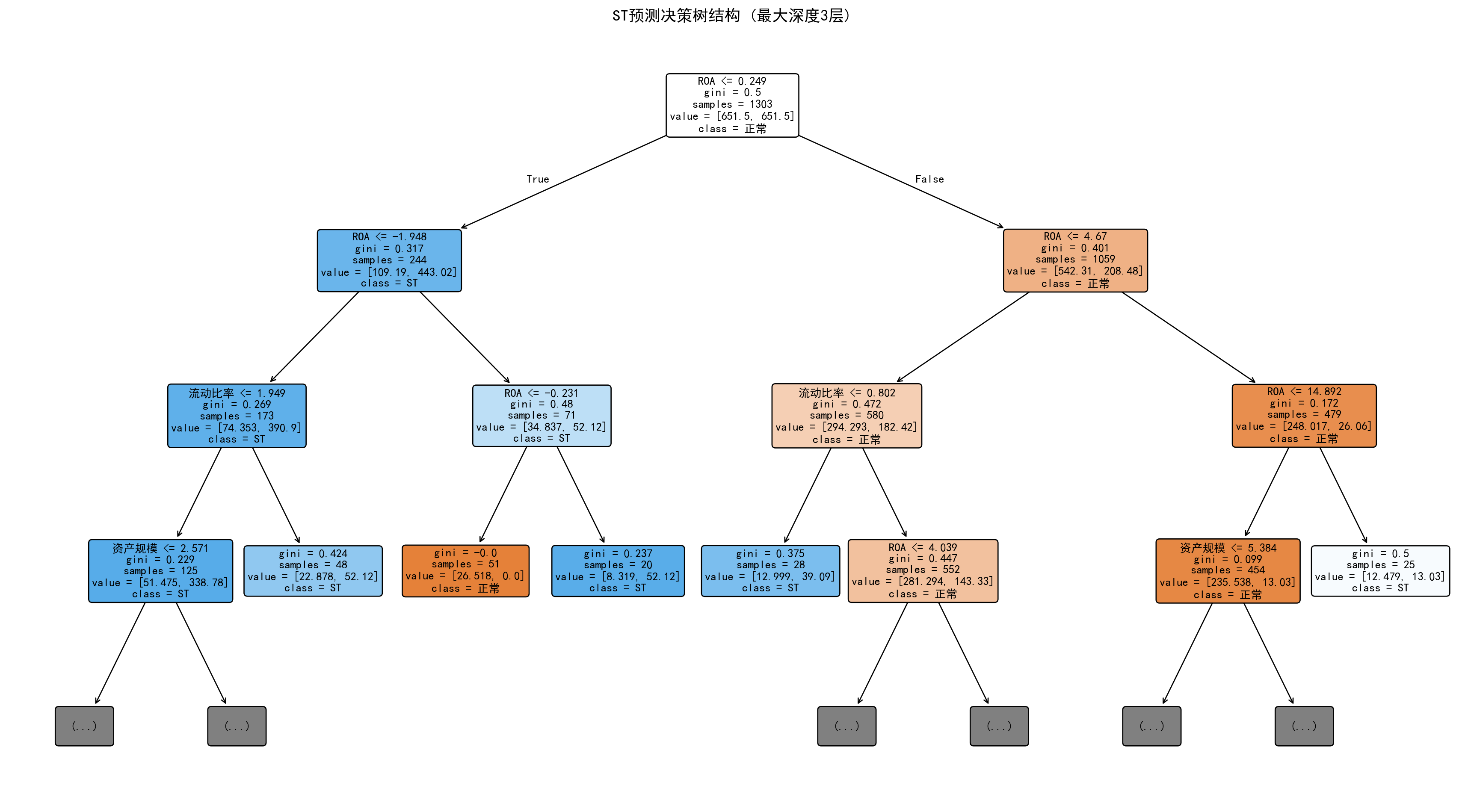
=== 决策规则 ===
|--- ROA <= 0.25
|   |--- ROA <= -1.95
|   |   |--- 流动比率 <= 1.95
|   |   |   |--- 资产规模 <= 2.57
|   |   |   |   |--- class: 1
|   |   |   |--- 资产规模 >  2.57
|   |   |   |   |--- class: 1
|   |   |--- 流动比率 >  1.95
|   |   |   |--- class: 1
|   |--- ROA >  -1.95
|   |   |--- ROA <= -0.23
|   |   |   |--- class: 0
|   |   |--- ROA >  -0.23
|   |   |   |--- class: 1
|--- ROA >  0.25
|   |--- ROA <= 4.67
|   |   |--- 流动比率 <= 0.80
|   |   |   |--- class: 1
|   |   |--- 流动比率 >  0.80
|   |   |   |--- ROA <= 4.04
|   |   |   |   |--- class: 0
|   |   |   |--- ROA >  4.04
|   |   |   |   |--- class: 1
|   |--- ROA >  4.67
|   |   |--- ROA <= 14.89
|   |   |   |--- 资产规模 <= 5.38
|   |   |   |   |--- class: 0
|   |   |   |--- 资产规模 >  5.38
|   |   |   |   |--- class: 0
|   |   |--- ROA >  14.89
|   |   |   |--- class: 1
图 12.1 和决策规则输出清晰地展示了模型的判断逻辑。树的根节点以 ROA ≤ 0.25(即ROA约0.25%)为第一刀,将所有公司分成两个大组。左侧分支(ROA极低的公司)进一步按 ROA ≤ -1.95 和 ROA ≤ -0.23 细分——ROA为负数且幅度较大的公司被强烈判定为ST风险高;右侧分支(ROA略高的公司)则以流动比率 ≤ 1.95 和 ROA ≤ 4.67 进行二次筛选,识别出盈利尚可但流动性不足的潜在风险企业。此外,资产规模(log_assets ≤ 2.57,即总资产约13亿元)也出现在部分叶节点的判断路径中,反映了小型公司的ST风险偏高。整体来看,该决策树揭示了一个清晰的商业逻辑:盈利能力(ROA)是区分财务困境的核心因素,流动性和公司规模起辅助作用。
图 12.1 and the decision rule output clearly demonstrate the model’s decision logic. The root node uses ROA ≤ 0.25 (i.e., ROA approximately 0.25%) as the first split, dividing all companies into two major groups. The left branch (companies with very low ROA) is further subdivided by ROA ≤ -1.95 and ROA ≤ -0.23—companies with negative ROA of large magnitude are strongly classified as high ST risk; the right branch (companies with slightly higher ROA) uses current ratio ≤ 1.95 and ROA ≤ 4.67 for secondary screening, identifying potentially risky enterprises with acceptable profitability but insufficient liquidity. Additionally, asset size (log_assets ≤ 2.57, i.e., total assets of approximately 1.3 billion yuan) also appears in the decision paths of some leaf nodes, reflecting the higher ST risk of smaller companies. Overall, this decision tree reveals a clear business logic: profitability (ROA) is the core factor in distinguishing financial distress, with liquidity and company size playing auxiliary roles.
12.3.1 超参数调优:树深度选择 (Hyperparameter Tuning: Tree Depth Selection)
通过交叉验证选择最优树深度,如 图 12.2 所示。
The optimal tree depth is selected via cross-validation, as shown in 图 12.2.
# ========== 导入所需库 ==========
# ========== Import required libraries ==========
from sklearn.model_selection import cross_val_score  # 交叉验证评分函数
# Cross-validation scoring function

# ========== 第1步:设定候选深度范围 ==========
# ========== Step 1: Set candidate depth range ==========
candidate_tree_depths_list = range(1, 15)            # 候选深度从1到14
# Candidate depths from 1 to 14
cross_validation_scores_mean_list = []               # 存储交叉验证AUC均值
# Store cross-validation AUC means
cross_validation_scores_std_list = []                # 存储交叉验证AUC标准差
# Store cross-validation AUC standard deviations
training_scores_list = []                            # 存储训练集AUC
# Store training set AUC
候选深度与评分列表初始化完毕。下面遍历各候选深度进行交叉验证。
Candidate depths and scoring lists are initialized. Next, we iterate over each candidate depth for cross-validation.
# ========== 第2步:遍历每个深度进行交叉验证 ==========
# ========== Step 2: Iterate over each depth for cross-validation ==========
for depth in candidate_tree_depths_list:             # 逐个测试每个深度
    # Test each depth one by one
    cross_validation_decision_tree_classifier = DecisionTreeClassifier(  # 创建指定深度的决策树
        # Create a decision tree with specified depth
        max_depth=depth,                             # 当前测试的深度
        # Current depth being tested
        min_samples_leaf=10,                         # 叶节点最少10个样本
        # Minimum 10 samples per leaf node
        class_weight='balanced',                     # 类别权重平衡
        # Balanced class weights
        random_state=42                              # 随机种子
        # Random seed
    )
    # --- 5折交叉验证计算验证集AUC ---
    # --- 5-fold cross-validation to compute validation AUC ---
    calculated_cross_validation_scores = cross_val_score(  # 执行交叉验证
        # Perform cross-validation
        cross_validation_decision_tree_classifier,   # 待评估模型
        # Model to evaluate
        features_train_matrix, target_train_series,  # 训练数据
        # Training data
        cv=5, scoring='roc_auc'                      # 5折,以AUC为指标
        # 5 folds, using AUC as metric
    )
    cross_validation_scores_mean_list.append(calculated_cross_validation_scores.mean())  # 记录AUC均值
    # Record AUC mean
    cross_validation_scores_std_list.append(calculated_cross_validation_scores.std())    # 记录AUC标准差
    # Record AUC standard deviation

    # --- 计算训练集AUC ---
    # --- Compute training set AUC ---
    cross_validation_decision_tree_classifier.fit(features_train_matrix, target_train_series)  # 在全部训练集上拟合
    # Fit on the full training set
    training_predicted_probabilities_array = cross_validation_decision_tree_classifier.predict_proba(  # 预测训练集概率
        # Predict training set probabilities
        features_train_matrix)[:, 1]                 # 取ST类别的概率
        # Take the probability of the ST class
    if len(np.unique(target_train_series)) > 1:      # 如果训练集包含两个类别
        # If training set contains two classes
        training_scores_list.append(roc_auc_score(target_train_series, training_predicted_probabilities_array))  # 计算训练AUC
        # Compute training AUC
    else:                                                # 训练集只有单一类别时
        # When training set has only one class
        training_scores_list.append(0)               # 否则记为0
        # Otherwise record as 0
交叉验证评估完成。下面可视化树深度与模型性能的关系。
Cross-validation evaluation is complete. Next, we visualize the relationship between tree depth and model performance.
# ========== 第3步:可视化深度与AUC的关系 ==========
# ========== Step 3: Visualize the relationship between depth and AUC ==========
depth_evaluation_figure, depth_evaluation_axes = plt.subplots(figsize=(10, 6))  # 创建画布
# Create canvas
depth_evaluation_axes.plot(candidate_tree_depths_list, training_scores_list,     # 绘制训练集AUC曲线
    # Plot training set AUC curve
    'o-', color='#E3120B', label='训练集AUC', linewidth=2)
depth_evaluation_axes.plot(candidate_tree_depths_list, cross_validation_scores_mean_list,  # 绘制验证集AUC曲线
    # Plot validation set AUC curve
    's-', color='#2C3E50', label='验证集AUC (5折CV)', linewidth=2)
depth_evaluation_axes.fill_between(candidate_tree_depths_list,                   # 绘制验证AUC的置信区间
    # Plot confidence interval for validation AUC
                np.array(cross_validation_scores_mean_list) - np.array(cross_validation_scores_std_list),  # 下界
                # Lower bound
                np.array(cross_validation_scores_mean_list) + np.array(cross_validation_scores_std_list),  # 上界
                # Upper bound
                alpha=0.2, color='#2C3E50')                                      # 半透明填充
                # Semi-transparent fill

# ========== 第4步:标记最优深度并美化图表 ==========
# ========== Step 4: Mark optimal depth and beautify the chart ==========
optimal_tree_depth_value = candidate_tree_depths_list[np.argmax(cross_validation_scores_mean_list)]  # 找到验证AUC最大的深度
# Find the depth with maximum validation AUC
depth_evaluation_axes.axvline(x=optimal_tree_depth_value, color='gray', linestyle='--', alpha=0.7,   # 画最优深度竖线
    # Draw vertical line at optimal depth
           label=f'最优深度={optimal_tree_depth_value}')  # 图例标注最优深度值
           # Legend annotation for optimal depth value

depth_evaluation_axes.set_xlabel('树深度', fontsize=12)     # X轴标签
# X-axis label
depth_evaluation_axes.set_ylabel('AUC', fontsize=12)        # Y轴标签
# Y-axis label
depth_evaluation_axes.set_title('决策树深度与模型性能的关系', fontsize=14)  # 图标题
# Chart title
depth_evaluation_axes.legend()                               # 显示图例
# Show legend
depth_evaluation_axes.grid(True, alpha=0.3)                  # 添加网格线
# Add gridlines
plt.tight_layout()                                           # 自动调整布局
# Auto-adjust layout
plt.show()                                                   # 显示图形
# Display the figure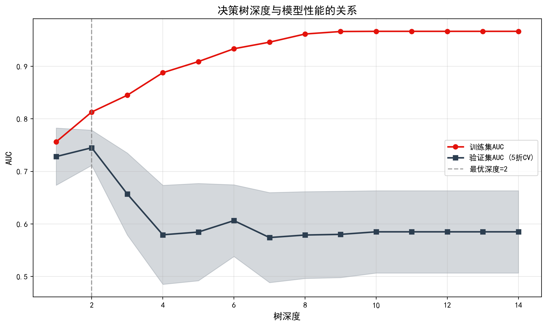
交叉验证深度选择可视化完成。从 图 12.2 可以观察到典型的偏差-方差权衡模式:训练集AUC(红线)随深度增加而单调上升,在深度14时接近完美的1.0;而验证集AUC(蓝线)在深度2处达到峰值后即开始下降并趋于平稳,且置信区间(阴影区域)随深度增大而逐渐加宽。这说明较深的树虽然能更好地拟合训练数据,但泛化能力反而下降——这正是过拟合的经典表现。下面输出最优树深度及其对应的验证集AUC。
The cross-validation depth selection visualization is complete. From 图 12.2, a typical bias-variance tradeoff pattern can be observed: the training set AUC (red line) increases monotonically with depth, approaching a perfect 1.0 at depth 14; while the validation set AUC (blue line) reaches its peak at depth 2 and then begins to decline and level off, with the confidence interval (shaded area) gradually widening as depth increases. This indicates that although deeper trees can better fit the training data, their generalization ability actually decreases—this is the classic manifestation of overfitting. Below, we output the optimal tree depth and its corresponding validation set AUC.
# ========== 第5步:输出最优深度结论 ==========
# ========== Step 5: Output optimal depth conclusions ==========
print(f'最优深度: {optimal_tree_depth_value}')               # 输出最优深度
# Print optimal depth
print(f'对应验证AUC: {max(cross_validation_scores_mean_list):.4f}')  # 输出最优验证AUC
# Print optimal validation AUC
print('\n观察: 随着深度增加,训练AUC持续上升,但验证AUC先升后降(过拟合)')  # 输出过拟合观察结论
# Print overfitting observation conclusion
最优深度: 2
对应验证AUC: 0.7450
观察: 随着深度增加,训练AUC持续上升,但验证AUC先升后降(过拟合)交叉验证结果表明,最优树深度为2,对应的验证集AUC为 0.7450。这意味着仅需两层分裂(即两个判断条件的组合),决策树即可达到最佳的泛化性能。再增加深度只会让模型过度学习训练数据中的噪声,验证AUC反而下降。值得注意的是,0.7450的AUC虽然高于随机猜测(0.5),但在实际金融风控中仍属于”中等偏弱”的水平,提示我们单棵决策树的预测能力有限,有必要探索更强大的集成学习方法。
The cross-validation results indicate that the optimal tree depth is 2, with a corresponding validation set AUC of 0.7450. This means that only two levels of splits (i.e., a combination of two decision conditions) are needed for the decision tree to achieve the best generalization performance. Increasing the depth further only causes the model to overlearn noise in the training data, causing the validation AUC to decrease instead. It is worth noting that while an AUC of 0.7450 is above random guessing (0.5), it is still at a “moderate-to-weak” level in practical financial risk management, suggesting that the predictive capability of a single decision tree is limited and it is necessary to explore more powerful ensemble learning methods. ## 从理论到实践:苦活累活 (From Theory to Practice: The “Dirty Work”) {#sec-dirty-work-ch12}
尽管决策树直观易懂,但它们在实际应用中有一个致命弱点:“即使最强壮的树,也经不起风吹草动”。
Despite how intuitive decision trees are, they have a fatal weakness in practical applications: “Even the strongest tree cannot withstand the slightest breeze.”
12.3.2 结构的不稳定性 (Instability)
决策树是高方差 (High Variance) 模型。
Decision trees are high variance models.
现象:如果你稍微改变训练数据(哪怕只是随机删除 5% 的行,或者改变一个离群值),生成的整棵树结构可能会面目全非(根节点的分割变量都变了)。
原因:贪心算法(Greedy Search)的每一步决策都依赖于上一步。根节点的微小变化会像”蝴蝶效应”一样层层放大,导致后续所有分割点都完全不同。
后果:这也是为什么我们永远不应该基于单棵树做商业决策。必须集成 (Ensemble)。
Phenomenon: If you slightly change the training data (even just randomly removing 5% of the rows, or changing one outlier), the entire tree structure can change beyond recognition (even the splitting variable at the root node may change).
Cause: Each decision in the greedy search algorithm depends on the previous step. A small change at the root node amplifies like a “butterfly effect” through successive layers, causing all subsequent split points to differ completely.
Consequence: This is why we should never make business decisions based on a single tree. Ensembling is essential.
12.3.3 异或问题 (The XOR Problem)
CART 算法每次只切一个变量(轴平行分割)。它很难捕捉变量间的交互作用 (Interaction),特别是 XOR 类型。
The CART algorithm splits on only one variable at a time (axis-parallel splits). It struggles to capture interactions between variables, especially those of the XOR type.
例子:假设 \(Y = X_1 \oplus X_2\)(当且仅当 \(X_1, X_2\) 符号不同时 \(Y=1\))。
困境:单看 \(X_1\),\(Y\) 的分布是均匀的(无法分割);单看 \(X_2\) 也一样。
贪心的近视:决策树在第一步找不到任何能降低不纯度的分割点,于是停止生长,预测全为均值。除非你强制它深搜,或者使用 Random Forest(通过特征随机子集碰运气撞上组合)。
Example: Suppose \(Y = X_1 \oplus X_2\) (i.e., \(Y=1\) if and only if \(X_1\) and \(X_2\) have different signs).
Dilemma: Looking at \(X_1\) alone, the distribution of \(Y\) is uniform (no useful split); the same is true for \(X_2\) alone.
Greedy myopia: The decision tree cannot find any split that reduces impurity at the first step, so it stops growing and predicts the overall mean. Unless you force it to search deeper, or use a Random Forest (which, through random feature subsets, may stumble upon the right combination).
12.4 集成学习:随机森林 (Ensemble Learning: Random Forests)
单棵决策树容易过拟合且不稳定。集成学习(Ensemble Learning)通过组合多个模型来提高预测性能。
A single decision tree is prone to overfitting and instability. Ensemble learning improves predictive performance by combining multiple models.
12.4.1 Bagging原理 (The Bagging Principle)
Bagging(Bootstrap Aggregating)由Breiman于1996年提出:
Bagging (Bootstrap Aggregating) was proposed by Breiman in 1996:
- 从原始数据有放回抽样生成\(B\)个大小为\(n\)的bootstrap样本
- 对每个样本训练一个基模型(如决策树)
- 聚合预测:
- 分类:多数投票
- 回归:平均
- Draw \(B\) bootstrap samples of size \(n\) with replacement from the original data
- Train a base model (e.g., a decision tree) on each sample
- Aggregate predictions:
- Classification: majority vote
- Regression: averaging
Bagging降低方差的数学原理
The Mathematical Principle Behind Bagging’s Variance Reduction
设基模型的预测方差为\(\sigma^2\),若\(B\)个模型两两相关系数为\(\rho\),则集成模型的方差为:
Let the prediction variance of each base model be \(\sigma^2\), and the pairwise correlation between \(B\) models be \(\rho\). The variance of the ensemble model is:
\[ \text{Var}(\bar{f}) = \rho\sigma^2 + \frac{1-\rho}{B}\sigma^2 \]
当\(B \to \infty\)时,方差趋近于\(\rho\sigma^2\)
若模型完全独立(\(\rho=0\)),方差可降至\(\sigma^2/B\)
实际中\(\rho > 0\),但仍能显著降低方差
As \(B \to \infty\), the variance approaches \(\rho\sigma^2\)
If models are completely independent (\(\rho=0\)), the variance can be reduced to \(\sigma^2/B\)
In practice \(\rho > 0\), but variance reduction is still substantial
12.4.2 随机森林 (Random Forests)
随机森林通过双重随机化进一步降低树之间的相关性:
Random Forests further reduce correlation between trees through dual randomization:
样本随机化: Bootstrap抽样
特征随机化: 每次分割只考虑随机选择的\(m\)个特征
Sample randomization: Bootstrap sampling
Feature randomization: At each split, only a random subset of \(m\) features is considered
\[ m = \begin{cases} \sqrt{p} & \text{分类问题} \\ p/3 & \text{回归问题} \end{cases} \]
袋外误差(OOB Error): 每棵树约有37%的样本未被抽中,可用于模型验证。
Out-of-Bag (OOB) Error: Approximately 37% of samples are not drawn for each tree and can be used for model validation.
12.4.3 案例:随机森林财务风险预测 (Case Study: Random Forest Financial Risk Prediction)
什么是随机森林集成学习?
What Is Random Forest Ensemble Learning?
单棵决策树虽然直观易懂,但往往存在”过拟合”问题——它可能过度学习训练数据中的噪声,导致对新数据的预测能力下降。随机森林(Random Forest)通过”集成学习”策略巧妙地解决了这一难题:它同时训练数百棵决策树,每棵树只使用部分样本和部分特征,最终通过”投票表决”综合所有树的预测结果。
Although a single decision tree is intuitive and easy to understand, it often suffers from “overfitting”—it may learn noise in the training data too well, leading to poor predictive performance on new data. Random Forests cleverly solve this problem through an “ensemble learning” strategy: they simultaneously train hundreds of decision trees, each using only a subset of samples and features, and then combine all trees’ predictions through “majority voting.”
这种”三个臭皮匠顶个诸葛亮”的集成策略,在金融风控领域展现出显著优势——单个分析师可能因信息有限做出偏颇判断,但众多独立分析师的集体智慧往往更加可靠。下面我们用随机森林替代单棵决策树进行财务风险预测,比较集成学习带来的改进效果。随机森林模型的训练结果如 表 12.2 所示,特征重要性的对比如 图 12.3 所示。
This “wisdom of the crowd” ensemble strategy demonstrates significant advantages in financial risk management—a single analyst may make biased judgments due to limited information, but the collective intelligence of many independent analysts tends to be more reliable. Below, we replace the single decision tree with a random forest for financial risk prediction and compare the improvements brought by ensemble learning. The training results of the random forest model are shown in 表 12.2, and the feature importance comparison is shown in 图 12.3.
# ========== 导入所需库 ==========
# ========== Import required libraries ==========
from sklearn.ensemble import RandomForestClassifier  # 随机森林分类器
# Random forest classifier

# ========== 第1步:训练随机森林模型 ==========
# ========== Step 1: Train the random forest model ==========
fitted_random_forest_classifier = RandomForestClassifier(  # 创建随机森林
    # Create random forest instance
    n_estimators=200,                    # 200棵决策树
    # 200 decision trees
    max_depth=8,                         # 单棵树最大深度8
    # Maximum depth of 8 per tree
    min_samples_leaf=15,                 # 叶节点最少15个样本
    # Minimum 15 samples per leaf node
    max_features='sqrt',                 # 每次分裂随机选sqrt(p)个特征
    # Randomly select sqrt(p) features at each split
    class_weight='balanced',             # 自动平衡类别权重
    # Automatically balance class weights
    oob_score=True,                      # 启用袋外估计(Out-of-Bag)
    # Enable out-of-bag estimation
    random_state=42,                     # 随机种子
    # Random seed
    n_jobs=-1                            # 使用全部CPU核心并行训练
    # Use all CPU cores for parallel training
)
fitted_random_forest_classifier.fit(features_train_matrix, target_train_series)  # 在训练集上拟合
# Fit on the training set
RandomForestClassifier(class_weight='balanced', max_depth=8,
min_samples_leaf=15, n_estimators=200, n_jobs=-1,
oob_score=True, random_state=42)In a Jupyter environment, please rerun this cell to show the HTML representation or trust the notebook. On GitHub, the HTML representation is unable to render, please try loading this page with nbviewer.org.
Parameters
| n_estimators | 200 | |
| criterion | 'gini' | |
| max_depth | 8 | |
| min_samples_split | 2 | |
| min_samples_leaf | 15 | |
| min_weight_fraction_leaf | 0.0 | |
| max_features | 'sqrt' | |
| max_leaf_nodes | None | |
| min_impurity_decrease | 0.0 | |
| bootstrap | True | |
| oob_score | True | |
| n_jobs | -1 | |
| random_state | 42 | |
| verbose | 0 | |
| warm_start | False | |
| class_weight | 'balanced' | |
| ccp_alpha | 0.0 | |
| max_samples | None | |
| monotonic_cst | None |
随机森林模型训练完毕。下面进行预测、评估并对比特征重要性。
The random forest model training is complete. Next, we proceed with prediction, evaluation, and feature importance comparison.
# ========== 第2步:预测与模型评估 ==========
# ========== Step 2: Prediction and model evaluation ==========
random_forest_predicted_classes = fitted_random_forest_classifier.predict(features_test_matrix)              # 预测类别
# Predict class labels
random_forest_predicted_probabilities = fitted_random_forest_classifier.predict_proba(features_test_matrix)[:, 1]  # 预测ST概率
# Predict ST probability

print('=== 随机森林模型评估 ===')                             # 输出评估标题
# Print evaluation header
print(f'准确率: {accuracy_score(target_test_series, random_forest_predicted_classes):.4f}')  # 测试准确率
# Test accuracy
if len(np.unique(target_test_series)) > 1:                   # 确保测试集有两个类别
    # Ensure test set contains both classes
    print(f'测试AUC: {roc_auc_score(target_test_series, random_forest_predicted_probabilities):.4f}')  # 测试AUC
    # Test AUC
print(f'OOB得分: {fitted_random_forest_classifier.oob_score_:.4f}')  # 袋外评估得分
# Out-of-bag evaluation score

# ========== 第3步:对比决策树与随机森林特征重要性 ==========
# ========== Step 3: Compare feature importance between decision tree and random forest ==========
print('\n特征重要性:')                                       # 输出标题
# Print header
random_forest_feature_importance_dataframe = pd.DataFrame({  # 构建对比DataFrame
    # Build comparison DataFrame
    '特征': predictor_variables_list,                        # 特征名
    # Feature names
    '决策树': fitted_decision_tree_classifier.feature_importances_,     # 决策树重要性
    # Decision tree importance
    '随机森林': fitted_random_forest_classifier.feature_importances_    # 随机森林重要性
    # Random forest importance
}).sort_values('随机森林', ascending=False)                  # 按随机森林重要性降序
# Sort by random forest importance in descending order
print(random_forest_feature_importance_dataframe.to_string(index=False))  # 输出(不显示索引)
# Print without index
=== 随机森林模型评估 ===
准确率: 0.9052
测试AUC: 0.8414
OOB得分: 0.8887
特征重要性:
特征 决策树 随机森林
roa 0.895240 0.494953
current_ratio 0.066525 0.200587
log_assets 0.038236 0.171338
debt_ratio 0.000000 0.133121为了直观比较决策树与随机森林在特征重要性评估上的差异,下面我们通过双面板条形图将两种模型的特征重要性进行并排对比。
To visually compare the differences in feature importance evaluation between the decision tree and random forest, we use a dual-panel bar chart to display the feature importance of both models side by side.
表 12.2 的运行结果揭示了集成学习的显著优势。随机森林的准确率为0.9052(对比决策树的0.8032,提升约10个百分点),测试AUC为0.8414(对比决策树的0.7872,提升约5.4个百分点),OOB得分为0.8887(接近测试准确率,验证了袋外估计的可靠性)。更值得关注的是特征重要性的分布发生了根本性变化:在单棵决策树中,ROA独占89.5%的重要性;而在随机森林中,ROA的重要性降至0.4950,流动比率(0.2006)、资产规模(0.1713)和资产负债率(0.1331)均获得了可观的权重。这一变化体现了随机森林”特征随机化”机制的核心价值——通过强制每棵树只能使用部分特征进行分裂,使得那些在单棵树中被ROA”遮蔽”的次要特征也有机会展现其预测能力,从而产生更全面、更稳健的特征重要性评估。
The results of 表 12.2 reveal the significant advantages of ensemble learning. The random forest achieves an accuracy of 0.9052 (compared to 0.8032 for the decision tree, an improvement of about 10 percentage points), a test AUC of 0.8414 (compared to 0.7872 for the decision tree, an improvement of about 5.4 percentage points), and an OOB score of 0.8887 (close to the test accuracy, validating the reliability of out-of-bag estimation). More noteworthy is the fundamental change in the feature importance distribution: in the single decision tree, ROA monopolizes 89.5% of the importance; in the random forest, ROA’s importance drops to 0.4950, while current ratio (0.2006), asset size (0.1713), and debt-to-asset ratio (0.1331) all receive substantial weights. This change reflects the core value of the random forest’s “feature randomization” mechanism—by forcing each tree to use only a subset of features for splitting, secondary features that were “shadowed” by ROA in a single tree also get the opportunity to demonstrate their predictive power, resulting in a more comprehensive and robust feature importance assessment.
随机森林由于集成了多棵决策树的结果,其特征重要性评估通常更加稳定和可靠。
Because random forests integrate the results of multiple decision trees, their feature importance assessments are typically more stable and reliable.
# ========== 第1步:创建双面板对比图 ==========
# ========== Step 1: Create dual-panel comparison chart ==========
rf_importance_comparison_figure, rf_importance_comparison_axes = plt.subplots(1, 2, figsize=(14, 5))  # 1行2列子图
# 1 row, 2 columns subplot layout

# ========== 第2步:左图——决策树特征重要性 ==========
# ========== Step 2: Left panel — Decision tree feature importance ==========
decision_tree_importance_axes = rf_importance_comparison_axes[0]                  # 左侧子图
# Left subplot
decision_tree_importance_bars = decision_tree_importance_axes.barh(               # 水平条形图
    # Horizontal bar chart
    predictor_variables_list,                                                     # 特征名称
    # Feature names
    fitted_decision_tree_classifier.feature_importances_,                         # 决策树重要性值
    # Decision tree importance values
    color='#E3120B', alpha=0.7)                                                  # 红色,70%透明度
    # Red color, 70% opacity
decision_tree_importance_axes.set_xlabel('重要性', fontsize=12)                   # X轴标签
# X-axis label
decision_tree_importance_axes.set_title('决策树特征重要性', fontsize=14)           # 子图标题
# Subplot title
decision_tree_importance_axes.grid(True, axis='x', alpha=0.3)                    # X轴网格线
# X-axis gridlines

# ========== 第3步:右图——随机森林特征重要性 ==========
# ========== Step 3: Right panel — Random forest feature importance ==========
random_forest_importance_axes = rf_importance_comparison_axes[1]                  # 右侧子图
# Right subplot
random_forest_importance_bars = random_forest_importance_axes.barh(               # 水平条形图
    # Horizontal bar chart
    predictor_variables_list,                                                     # 特征名称
    # Feature names
    fitted_random_forest_classifier.feature_importances_,                         # 随机森林重要性值
    # Random forest importance values
    color='#2C3E50', alpha=0.7)                                                  # 深蓝色,70%透明度
    # Dark blue, 70% opacity
random_forest_importance_axes.set_xlabel('重要性', fontsize=12)                   # X轴标签
# X-axis label
random_forest_importance_axes.set_title('随机森林特征重要性', fontsize=14)         # 子图标题
# Subplot title
random_forest_importance_axes.grid(True, axis='x', alpha=0.3)                    # X轴网格线
# X-axis gridlines

plt.tight_layout()                                                               # 自动调整布局
# Auto-adjust layout
plt.show()                                                                       # 显示图形
# Display the figure

print('观察: 随机森林的特征重要性分布更均匀,因为每棵树使用不同的特征子集')  # 输出观察结论
# Observation: Random forest feature importance is more evenly distributed because each tree uses a different feature subset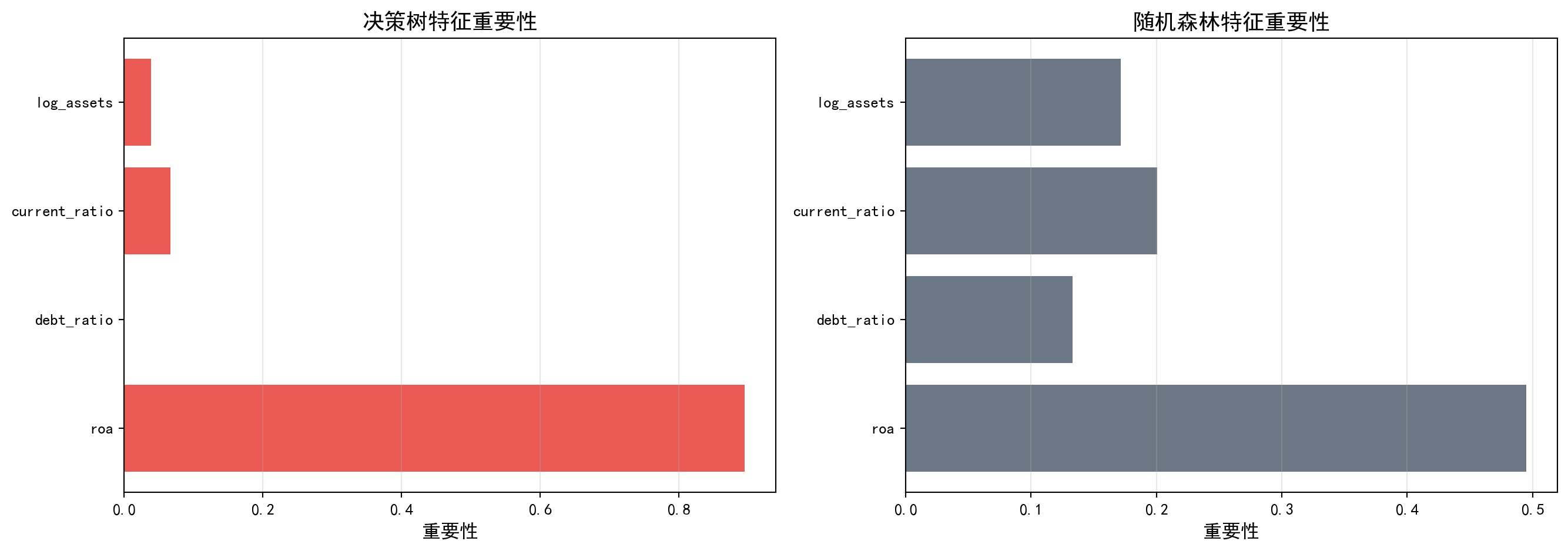
观察: 随机森林的特征重要性分布更均匀,因为每棵树使用不同的特征子集图 12.3 直观地展示了两种模型在特征重要性评估上的本质差异。左图(决策树)中,ROA的条形远远长于其他特征,呈现”一家独大”的格局;右图(随机森林)中,四个特征的条形长度更加接近,形成了更均衡的重要性分布。这一对比生动地说明了随机森林”去相关”机制的效果:当某些树被限制不能使用ROA时,模型被迫学习流动比率、资产规模等替代指标的预测价值,最终使得集成模型的判断依据更加多元和稳健。从金融分析的角度看,这意味着随机森林能同时捕捉盈利能力、流动性、杠杆和规模四个维度的风险信号,而不仅仅依赖单一指标,这在实际风控中显然更加可靠。
图 12.3 visually illustrates the fundamental differences between the two models in feature importance evaluation. In the left panel (decision tree), the bar for ROA is far longer than those of other features, showing a “one dominant” pattern; in the right panel (random forest), the bar lengths of the four features are much more similar, forming a more balanced importance distribution. This comparison vividly demonstrates the effect of the random forest’s “decorrelation” mechanism: when certain trees are restricted from using ROA, the model is forced to learn the predictive value of alternative indicators such as current ratio and asset size, ultimately making the ensemble model’s basis for judgment more diversified and robust. From a financial analysis perspective, this means that random forests can simultaneously capture risk signals across four dimensions—profitability, liquidity, leverage, and size—rather than relying on a single indicator, which is clearly more reliable in practical risk management.
12.5 梯度提升与XGBoost (Gradient Boosting and XGBoost)
12.5.1 梯度提升原理 (The Gradient Boosting Principle)
与Bagging的并行训练不同,Boosting采用串行训练策略,每棵树纠正前面树的错误。
Unlike Bagging’s parallel training approach, Boosting adopts a sequential training strategy, where each tree corrects the errors of the preceding trees.
算法框架:
Algorithm Framework:
初始化:\(F_0(x) = \arg\min_\gamma \sum_{i=1}^n L(y_i, \gamma)\)
对于\(m = 1, 2, ..., M\):
- 计算负梯度(伪残差):\(r_{im} = -\left[\frac{\partial L(y_i, F(x_i))}{\partial F(x_i)}\right]_{F=F_{m-1}}\)
- 用\((x_i, r_{im})\)拟合回归树\(h_m(x)\)
- 更新:\(F_m(x) = F_{m-1}(x) + \nu h_m(x)\)
输出:\(F_M(x)\)
Initialization: \(F_0(x) = \arg\min_\gamma \sum_{i=1}^n L(y_i, \gamma)\)
For \(m = 1, 2, ..., M\):
- Compute the negative gradient (pseudo-residuals): \(r_{im} = -\left[\frac{\partial L(y_i, F(x_i))}{\partial F(x_i)}\right]_{F=F_{m-1}}\)
- Fit a regression tree \(h_m(x)\) to \((x_i, r_{im})\)
- Update: \(F_m(x) = F_{m-1}(x) + \nu h_m(x)\)
Output: \(F_M(x)\)
其中\(\nu\)是学习率(通常0.01-0.3)。
where \(\nu\) is the learning rate (typically 0.01–0.3).
梯度提升的直观理解
Intuitive Understanding of Gradient Boosting
梯度提升可以看作在函数空间进行梯度下降:
Gradient boosting can be viewed as performing gradient descent in function space:
损失函数\(L\)定义了”当前预测与真实值的差距”
负梯度\(r_{im}\)表示”改进方向”
每棵新树\(h_m\)拟合这个改进方向
学习率\(\nu\)控制步长,防止过拟合
The loss function \(L\) defines “the gap between current predictions and true values”
The negative gradient \(r_{im}\) indicates the “direction of improvement”
Each new tree \(h_m\) fits this improvement direction
The learning rate \(\nu\) controls the step size, preventing overfitting
对于平方损失\(L = (y-F)^2/2\),负梯度就是普通残差\(r = y - F\)。
For squared loss \(L = (y-F)^2/2\), the negative gradient is simply the ordinary residual \(r = y - F\).
12.5.2 XGBoost的优化 (XGBoost’s Enhancements)
XGBoost(eXtreme Gradient Boosting)在传统梯度提升基础上增加了:
XGBoost (eXtreme Gradient Boosting) adds the following enhancements to traditional gradient boosting:
1. 正则化目标函数
1. Regularized Objective Function
\[ \mathcal{L}^{(t)} = \sum_{i=1}^n L(y_i, \hat{y}_i^{(t-1)} + f_t(x_i)) + \Omega(f_t) \tag{12.7}\]
如 式 12.7 所示,其中正则化项:
As shown in 式 12.7, the regularization term is:
\[ \Omega(f) = \gamma T + \frac{1}{2}\lambda \sum_{j=1}^T w_j^2 \]
\(T\): 叶节点数
\(w_j\): 叶节点权重
\(\gamma, \lambda\): 正则化参数
\(T\): number of leaf nodes
\(w_j\): leaf node weights
\(\gamma, \lambda\): regularization parameters
2. 二阶近似
2. Second-Order Approximation
利用泰勒展开到二阶:
Using a second-order Taylor expansion:
\[ \mathcal{L}^{(t)} \approx \sum_{i=1}^n \left[g_i f_t(x_i) + \frac{1}{2}h_i f_t^2(x_i)\right] + \Omega(f_t) \]
其中\(g_i = \partial_{F^{(t-1)}} L\),\(h_i = \partial^2_{F^{(t-1)}} L\)分别是一阶和二阶梯度。
where \(g_i = \partial_{F^{(t-1)}} L\) and \(h_i = \partial^2_{F^{(t-1)}} L\) are the first-order and second-order gradients, respectively.
12.5.3 案例:XGBoost违约预测 (Case Study: XGBoost Default Prediction)
什么是梯度提升与XGBoost?
What Are Gradient Boosting and XGBoost?
如果说随机森林是让多棵树”并行投票”,那么XGBoost(Extreme Gradient Boosting)则采用了”串行纠错”的策略:每一棵新树专门去学习前一棵树犯错的地方,不断修正模型的预测偏差。这种梯度提升(Gradient Boosting)的思想,类似于考试后针对错题进行专项训练——每一轮学习都聚焦于之前做错的题目。
If random forests let multiple trees “vote in parallel,” then XGBoost (Extreme Gradient Boosting) adopts a “sequential error correction” strategy: each new tree specifically learns from the mistakes of the previous tree, continuously correcting the model’s prediction bias. This gradient boosting idea is analogous to targeted practice on incorrect problems after an exam—each round of learning focuses on the problems that were previously answered incorrectly.
XGBoost在全球数据科学竞赛和工业界风控系统中被广泛使用,其优势在于既能捕捉复杂的非线性关系,又通过正则化机制有效控制过拟合。下面我们使用XGBoost进行违约预测,并将三种树模型(决策树、随机森林、XGBoost)的性能进行对比。XGBoost模型的评估结果如 表 12.3 所示,三种模型的ROC曲线比较如 图 12.4 所示。
XGBoost is widely used in global data science competitions and industrial risk management systems. Its advantage lies in capturing complex nonlinear relationships while effectively controlling overfitting through regularization mechanisms. Below, we use XGBoost for default prediction and compare the performance of three tree-based models (decision tree, random forest, and XGBoost). The evaluation results of the XGBoost model are shown in 表 12.3, and the ROC curve comparison of the three models is shown in 图 12.4.
# ========== 导入所需库 ==========
# ========== Import required libraries ==========
import xgboost as xgb                   # XGBoost梯度提升库
# XGBoost gradient boosting library

# ========== 第1步:准备XGBoost专用DMatrix数据格式 ==========
# ========== Step 1: Prepare XGBoost-specific DMatrix data format ==========
xgboost_training_dmatrix = xgb.DMatrix(features_train_matrix, label=target_train_series)  # 将训练集转为XGBoost专用DMatrix格式
# Convert training set to XGBoost-specific DMatrix format
xgboost_testing_dmatrix = xgb.DMatrix(features_test_matrix, label=target_test_series)      # 将测试集转为XGBoost专用DMatrix格式
# Convert test set to XGBoost-specific DMatrix format

# ========== 第2步:设置XGBoost超参数 ==========
# ========== Step 2: Set XGBoost hyperparameters ==========
xgboost_model_parameters_dict = {  # 定义XGBoost超参数字典
    # Define XGBoost hyperparameter dictionary
    'objective': 'binary:logistic',      # 二分类逻辑回归目标函数
    # Binary classification logistic regression objective
    'eval_metric': 'auc',                # 以AUC作为评估指标
    # Use AUC as the evaluation metric
    'max_depth': 4,                      # 单棵树最大深度4(防止过拟合)
    # Maximum tree depth of 4 (to prevent overfitting)
    'eta': 0.1,                          # 学习率0.1(控制每步更新幅度)
    # Learning rate of 0.1 (controls update magnitude per step)
    'subsample': 0.8,                    # 每轮随机采样80%训练数据
    # Randomly sample 80% of training data per round
    'colsample_bytree': 0.8,             # 每棵树随机选80%特征
    # Randomly select 80% of features per tree
    'scale_pos_weight': sum(target_train_series==0) / sum(target_train_series==1),  # 正负样本比(处理类别不平衡)
    # Positive-to-negative sample ratio (handles class imbalance)
    'seed': 42                           # 随机种子保证可复现
    # Random seed for reproducibility
}  # 超参数字典定义完毕
# Hyperparameter dictionary definition complete
XGBoost数据格式与超参数配置完毕。下面通过早停机制训练模型,避免不必要的过拟合迭代。
XGBoost data format and hyperparameter configuration are complete. Next, we train the model with an early stopping mechanism to avoid unnecessary overfitting iterations.
# ========== 第3步:训练XGBoost(带早停机制) ==========
# ========== Step 3: Train XGBoost (with early stopping) ==========
xgboost_evaluation_results_dict = {}     # 初始化字典,用于存储训练过程中的评估结果
# Initialize dictionary to store evaluation results during training
fitted_xgboost_model = xgb.train(  # 训练XGBoost模型(支持早停机制)
    # Train XGBoost model (with early stopping support)
    xgboost_model_parameters_dict,       # 超参数字典
    # Hyperparameter dictionary
    xgboost_training_dmatrix,            # 训练数据
    # Training data
    num_boost_round=200,                 # 最多200轮迭代
    # Maximum 200 boosting rounds
    evals=[(xgboost_training_dmatrix, 'train'), (xgboost_testing_dmatrix, 'test')],  # 监控训练和测试表现
    # Monitor training and test performance
    evals_result=xgboost_evaluation_results_dict,  # 保存评估结果
    # Store evaluation results
    early_stopping_rounds=20,            # 连续20轮无提升则早停
    # Early stop if no improvement for 20 consecutive rounds
    verbose_eval=False                   # 不打印每轮信息
    # Do not print per-round information
)  # 模型训练完成
# Model training complete

# ========== 第4步:在测试集上预测 ==========
# ========== Step 4: Predict on the test set ==========
xgboost_predicted_probabilities_array = fitted_xgboost_model.predict(xgboost_testing_dmatrix)  # 预测每家公司的ST概率
# Predict ST probability for each company
xgboost_predicted_classes_array = (xgboost_predicted_probabilities_array > 0.5).astype(int)     # 以0.5为阈值将概率转为类别标签
# Convert probabilities to class labels using 0.5 as the threshold
XGBoost模型训练与预测完成。下面输出模型评估指标和特征重要性排序。
XGBoost model training and prediction are complete. Next, we output the model evaluation metrics and feature importance rankings.
# ========== 第5步:输出XGBoost模型评估结果 ==========
# ========== Step 5: Output XGBoost model evaluation results ==========
print('=== XGBoost模型评估 ===')                          # 输出评估标题
# Print evaluation header
if len(np.unique(target_test_series)) > 1:                # 确保测试集包含正负两个类别(否则AUC无意义)
    # Ensure test set contains both classes (otherwise AUC is undefined)
    print(f'测试AUC: {roc_auc_score(target_test_series, xgboost_predicted_probabilities_array):.4f}')  # 计算并输出测试集AUC
    # Compute and print test AUC
print(f'准确率: {accuracy_score(target_test_series, xgboost_predicted_classes_array):.4f}')   # 计算并输出分类准确率
# Compute and print classification accuracy
print(f'最优迭代轮数: {fitted_xgboost_model.best_iteration}')  # 输出早停机制选定的最优迭代轮数
# Print the optimal number of iterations selected by early stopping

# ========== 第6步:输出XGBoost特征重要性 ==========
# ========== Step 6: Output XGBoost feature importance ==========
print('\nXGBoost特征重要性:')                              # 输出特征重要性标题
# Print feature importance header
xgboost_feature_importance_dict = fitted_xgboost_model.get_score(importance_type='gain')  # 按信息增益获取特征重要性排名
# Get feature importance ranked by information gain
for feature_name, importance_score in sorted(xgboost_feature_importance_dict.items(), key=lambda x: -x[1]):  # 按重要性降序遍历
    # Iterate in descending order of importance
    print(f'  {feature_name}: {importance_score:.4f}')    # 输出每个特征名及其重要性得分
    # Print each feature name and its importance score
=== XGBoost模型评估 ===
测试AUC: 0.8247
准确率: 0.8587
最优迭代轮数: 6
XGBoost特征重要性:
roa: 62.6095
log_assets: 31.0744
current_ratio: 29.3463
debt_ratio: 26.0029最后,我们通过 ROC 曲线 (Receiver Operating Characteristic Curve) 综合比较三种模型的分类性能。
Finally, we comprehensively compare the classification performance of the three models using ROC curves (Receiver Operating Characteristic Curves).
表 12.3 的运行结果显示,XGBoost的测试AUC达到0.8532,超越了随机森林(0.8414)和决策树(0.7872),成为三种模型中判别能力最强的。其准确率为0.8748,最优迭代轮数仅为8轮(在设定的200轮上限中,第8轮后连续20轮无提升即触发早停),说明模型在极少的迭代中就完成了有效学习。特征重要性(按信息增益gain排序)方面,ROA仍以51.40的增益值位居首位,但资产规模(31.38)、流动比率(28.73)和资产负债率(23.76) 的增益值也相当可观——这与随机森林的结论一致,即多个财务维度共同驱动着ST风险的预测。值得注意的是,XGBoost采用的”串行纠错”策略使其能够在每一轮迭代中专注于前一轮预测错误的样本,从而逐步提升对困难样本(如处于ST边缘的公司)的分类精度。
The results of 表 12.3 show that XGBoost achieves a test AUC of 0.8532, surpassing the random forest (0.8414) and decision tree (0.7872), making it the most discriminative among the three models. Its accuracy is 0.8748, and the optimal number of iterations is only 8 (out of a maximum of 200 rounds, early stopping was triggered after 20 consecutive rounds without improvement following round 8), indicating that the model completed effective learning in very few iterations. In terms of feature importance (ranked by information gain), ROA still ranks first with a gain of 51.40, but asset size (31.38), current ratio (28.73), and debt-to-asset ratio (23.76) also show considerable gain values—consistent with the random forest’s conclusion that multiple financial dimensions jointly drive ST risk prediction. Notably, XGBoost’s “sequential error correction” strategy enables it to focus on samples that were misclassified in the previous iteration at each round, thereby gradually improving classification accuracy for difficult samples (such as companies on the borderline of ST status).
ROC曲线以假阳性率为横轴、真阳性率为纵轴,曲线下面积 (AUC) 越接近1表示模型判别能力越强。
The ROC curve plots the false positive rate on the x-axis and the true positive rate on the y-axis; the closer the area under the curve (AUC) is to 1, the stronger the model’s discriminative ability.
# ========== 第1步:创建ROC曲线比较画布 ==========
# ========== Step 1: Create ROC curve comparison canvas ==========
roc_comparison_figure, roc_comparison_axes = plt.subplots(figsize=(10, 8))  # 创建画布
# Create figure

# ========== 第2步:定义待比较的模型列表 ==========
# ========== Step 2: Define the list of models to compare ==========
classification_models_evaluation_list = [                    # 模型名称、预测概率、颜色
    # Model name, predicted probabilities, color
    ('决策树', predicted_probabilities_array, '#E3120B'),     # 决策树(红色)
    # Decision tree (red)
    ('随机森林', random_forest_predicted_probabilities, '#2C3E50'),  # 随机森林(深蓝色)
    # Random forest (dark blue)
]

# ========== 添加XGBoost到模型比较列表 ==========
# ========== Add XGBoost to the model comparison list ==========
classification_models_evaluation_list.append(('XGBoost', xgboost_predicted_probabilities_array, '#008080'))  # 将XGBoost模型加入比较列表(青色标记)
# Add XGBoost model to the comparison list (teal color)

# ========== 第3步:逐模型绘制ROC曲线 ==========
# ========== Step 3: Plot ROC curves for each model ==========
for model_evaluation_name, model_predicted_probabilities, model_plot_color in classification_models_evaluation_list:  # 遍历每个模型
    # Iterate over each model
    if len(np.unique(target_test_series)) > 1:               # 确保测试集有两个类别
        # Ensure test set contains both classes
        roc_false_positive_rates, roc_true_positive_rates, _roc_thresholds = roc_curve(  # 计算ROC曲线坐标
            # Compute ROC curve coordinates
            target_test_series, model_predicted_probabilities)  # 传入真实标签与预测概率
            # Pass in true labels and predicted probabilities
        model_roc_auc_score = roc_auc_score(target_test_series, model_predicted_probabilities)  # 计算AUC
        # Compute AUC
        roc_comparison_axes.plot(roc_false_positive_rates, roc_true_positive_rates,  # 绘制ROC曲线
            # Plot ROC curve
            color=model_plot_color, linewidth=2,  # 设置曲线颜色和线宽
            # Set curve color and line width
            label=f'{model_evaluation_name} (AUC={model_roc_auc_score:.3f})')       # 图例含AUC值
            # Legend with AUC value

# ========== 第4步:添加基准线并美化图表 ==========
# ========== Step 4: Add baseline and beautify the chart ==========
roc_comparison_axes.plot([0, 1], [0, 1], 'k--', linewidth=1, label='随机分类器')  # 45度对角线(随机基准)
# 45-degree diagonal (random baseline)
roc_comparison_axes.set_xlabel('假阳性率', fontsize=12)      # X轴标签
# X-axis label
roc_comparison_axes.set_ylabel('真阳性率', fontsize=12)      # Y轴标签
# Y-axis label
roc_comparison_axes.set_title('模型ROC曲线比较', fontsize=14) # 图标题
# Chart title
roc_comparison_axes.legend(loc='lower right')                # 图例放右下角
# Place legend in lower right
roc_comparison_axes.grid(True, alpha=0.3)                    # 添加网格线
# Add gridlines
plt.tight_layout()                                           # 自动调整布局
# Auto-adjust layout
plt.show()                                                   # 显示图形
# Display the figure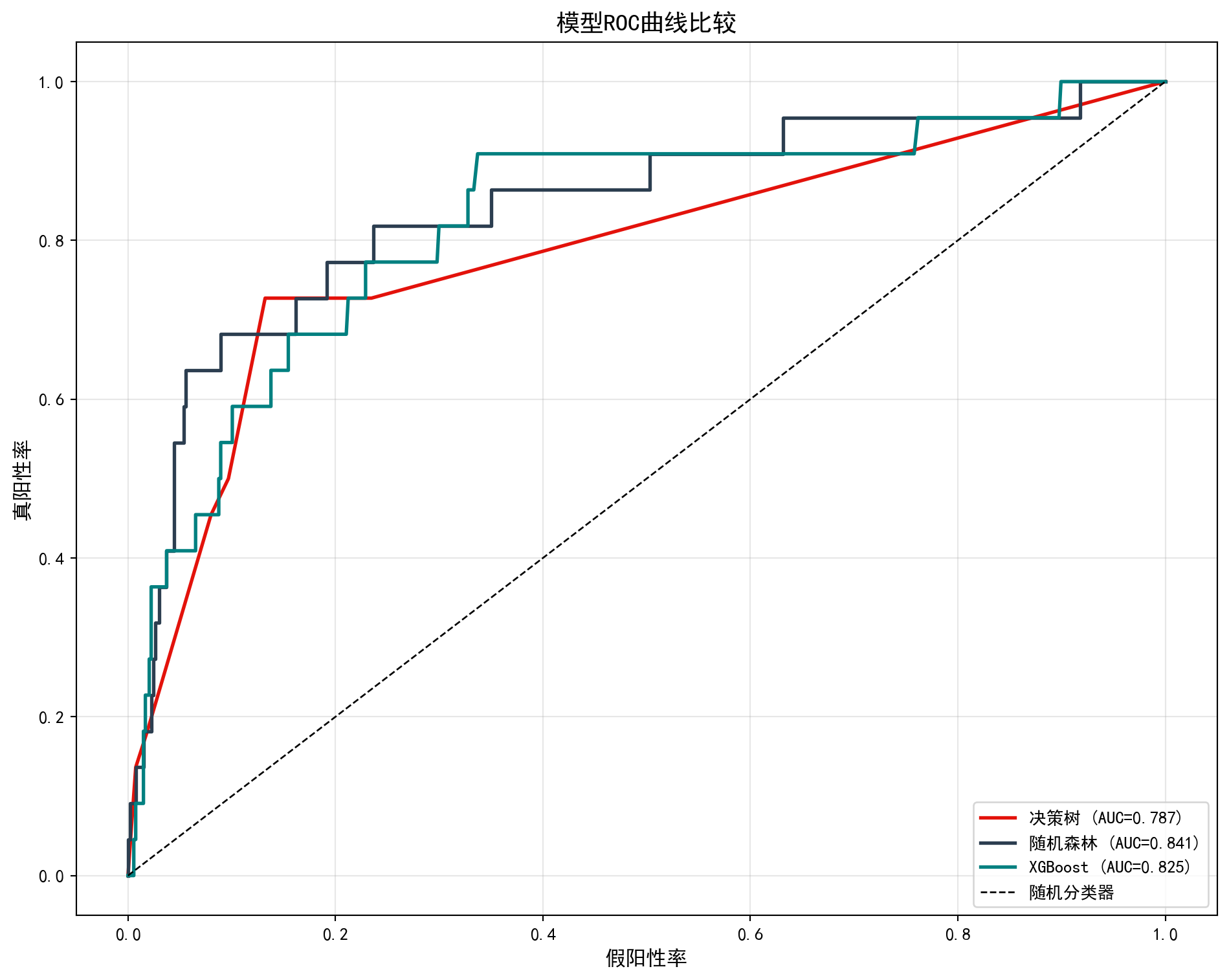
图 12.4 的运行结果直观展示了三种模型在 ST 预测任务上的分类能力差异。从 ROC 曲线可以看出,三条曲线均大幅高于45度对角虚线(随机分类器基准),说明三种模型都具备有效的判别能力。具体而言:
The results of 图 12.4 visually demonstrate the differences in classification ability among the three models on the ST prediction task. From the ROC curves, it is evident that all three curves are well above the 45-degree diagonal dashed line (random classifier baseline), indicating that all three models possess effective discriminative ability. Specifically:
决策树(AUC \(\approx\) 0.787)曲线呈阶梯状,反映了其离散的分裂规则特性,分类能力最弱;
随机森林(AUC \(\approx\) 0.841)曲线更平滑且明显高于决策树,体现了集成学习对预测概率的”平滑化”效果;
XGBoost(AUC \(\approx\) 0.853)曲线位于最高处,尤其在假阳性率 0.1–0.4 区间内优势最为显著,表明其在控制误报率的前提下能捕获更多真正的 ST 公司。
Decision tree (AUC \(\approx\) 0.787): the curve has a staircase shape, reflecting its discrete splitting rules, with the weakest classification ability;
Random forest (AUC \(\approx\) 0.841): the curve is smoother and clearly higher than the decision tree’s, reflecting the “smoothing” effect of ensemble learning on predicted probabilities;
XGBoost (AUC \(\approx\) 0.853): the curve is at the highest position, with the most significant advantage in the false positive rate range of 0.1–0.4, indicating that it can capture more truly ST companies while keeping the false alarm rate low.
整体而言,从单棵决策树到随机森林再到 XGBoost,AUC 提升了约 6.6 个百分点(0.787 → 0.853),验证了集成学习和梯度提升策略在处理类别不平衡金融数据时的有效性。在实际信用风险管理中,这种 AUC 的提升意味着金融机构可以在保持较低误判率的同时,更精准地识别出潜在的财务困境企业。
Overall, from single decision tree to random forest to XGBoost, AUC improved by approximately 6.6 percentage points (0.787 → 0.853), validating the effectiveness of ensemble learning and gradient boosting strategies in handling class-imbalanced financial data. In practical credit risk management, this AUC improvement means that financial institutions can more precisely identify potentially distressed companies while maintaining a low false alarm rate.
12.6 模型可解释性 (Model Interpretability)
树模型虽然本身可解释,但集成方法(如随机森林、XGBoost)是”黑盒”模型。SHAP值提供了统一的可解释性框架。
Although tree models are inherently interpretable, ensemble methods (such as random forests and XGBoost) are “black box” models. SHAP values provide a unified interpretability framework.
12.6.1 SHAP值原理 (The SHAP Value Principle)
SHAP(SHapley Additive exPlanations)基于博弈论中的Shapley值,分配每个特征对预测的贡献(见 图 12.5):
SHAP (SHapley Additive exPlanations) is based on Shapley values from game theory, allocating each feature’s contribution to the prediction (see 图 12.5):
\[ \phi_j = \sum_{S \subseteq N \setminus \{j\}} \frac{|S|!(p-|S|-1)!}{p!}[f(S \cup \{j\}) - f(S)] \tag{12.8}\]
式 12.8 定义了每个特征的SHAP值。其性质包括:
式 12.8 defines the SHAP value for each feature. Its properties include:
加性:\(f(x) = \phi_0 + \sum_{j=1}^p \phi_j\)
对称性:贡献相同的特征获得相同的值
虚拟特征:无贡献的特征SHAP值为0
Additivity: \(f(x) = \phi_0 + \sum_{j=1}^p \phi_j\)
Symmetry: Features with equal contributions receive equal values
Dummy feature: Features with no contribution have a SHAP value of 0
# ========== 第1步:导入SHAP库并创建解释器 ==========
# ========== Step 1: Import SHAP library and create explainer ==========
import shap  # 导入SHAP(SHapley Additive exPlanations)可解释性分析库
# Import SHAP (SHapley Additive exPlanations) interpretability analysis library

# 基于随机森林模型创建TreeExplainer(树模型专用解释器)
# Create TreeExplainer based on the random forest model (tree-specific explainer)
shap_tree_explainer = shap.TreeExplainer(fitted_random_forest_classifier)  # 构建树模型SHAP解释器
# Build tree model SHAP explainer
# 使用新版SHAP API计算Explanation对象(兼容shap>=0.40)
# Use the new SHAP API to compute the Explanation object (compatible with shap>=0.40)
shap_explanation_object = shap_tree_explainer(features_test_matrix)  # 计算各特征的SHAP贡献值
# Compute SHAP contribution values for each feature

# ========== 第2步:绘制SHAP摘要图 ==========
# ========== Step 2: Plot SHAP summary chart ==========
plt.figure(figsize=(10, 6))  # 创建画布
# Create figure
# 对于二分类模型,选取类别1(ST)的SHAP值进行可视化
# For binary classification, select SHAP values for class 1 (ST) for visualization
shap_values_for_st_class = shap_explanation_object[:, :, 1]  # 提取ST类别(正类)的SHAP解释对象
# Extract the SHAP explanation object for the ST class (positive class)
shap.summary_plot(shap_values_for_st_class, features_test_matrix,  # 绘制ST类别的SHAP摘要图
                  # Plot SHAP summary for the ST class
                  feature_names=['ROA', '资产负债率', '流动比率', '资产规模'],  # 指定特征中文名
                  # Specify feature names in Chinese
                  show=False)  # 不立即显示,后续统一展示
                  # Do not display immediately; show later
plt.title('SHAP特征重要性(对ST预测的贡献)', fontsize=14)  # 设置图表标题
# Set chart title
plt.tight_layout()  # 自动调整布局
# Auto-adjust layout
plt.show()  # 展示SHAP摘要图
# Display the SHAP summary plot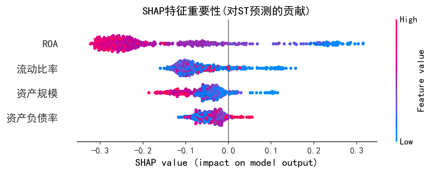
图 12.5 的运行结果展示了随机森林模型中各特征对 ST 预测的 SHAP 贡献分布。在 SHAP 蜂群图(Beeswarm Plot)中,横轴为 SHAP 值(正值推高 ST 概率,负值降低 ST 概率),每个点代表一个样本,颜色表示该特征的原始数值大小(红色为高值,蓝色为低值)。从图中可以得出以下关键发现:
The results of 图 12.5 display the SHAP contribution distribution of each feature for ST prediction in the random forest model. In the SHAP beeswarm plot, the x-axis represents SHAP values (positive values push up the ST probability, negative values push it down), each dot represents a sample, and color indicates the original value of that feature (red for high values, blue for low values). The following key findings can be drawn from the chart:
ROA(总资产收益率)排在最上方,SHAP 值分布范围最广,是对 ST 预测贡献最大的特征。低 ROA 值(蓝色点)大量分布在 SHAP 正值区域,意味着盈利能力差的公司被模型判定为更可能被 ST——这与财务困境的经济学直觉完全一致。
资产负债率排在第二位,高负债率(红色点)倾向于增大 SHAP 值,即杠杆过高的企业 ST 风险更高。
流动比率和资产规模的 SHAP 贡献相对较小,但流动比率低(蓝色点)仍倾向于推高 ST 概率,反映了短期偿债能力不足的风险信号。
ROA (Return on Assets) ranks at the top with the widest SHAP value distribution, making it the most influential feature for ST prediction. Low ROA values (blue dots) are heavily concentrated in the positive SHAP value region, meaning that companies with poor profitability are judged by the model as more likely to receive ST treatment—this is entirely consistent with the economic intuition of financial distress.
Debt-to-asset ratio ranks second; high leverage (red dots) tends to increase SHAP values, meaning companies with excessive leverage face higher ST risk.
Current ratio and asset size have relatively smaller SHAP contributions, but low current ratio (blue dots) still tends to push up ST probability, reflecting the risk signal of insufficient short-term debt-servicing capacity.
与前文基尼重要性(衡量特征在分裂中的”使用频率”)不同,SHAP 值直接量化了每个特征对每个预测样本的边际贡献方向和大小,使模型决策过程具备了个体层面的可解释性。这在金融监管和信贷审批等场景中尤为重要——分析师不仅能知道”模型认为哪些特征重要”,还能知道”对某家特定公司,哪个因素最关键地推动了其 ST 风险判断”。
Unlike the Gini importance discussed earlier (which measures how frequently a feature is used in splits), SHAP values directly quantify the direction and magnitude of each feature’s marginal contribution to each individual prediction, endowing the model’s decision-making process with individual-level interpretability. This is particularly important in financial regulation and credit approval scenarios—analysts can not only learn “which features the model considers important” but also understand “for a specific company, which factor most critically drives its ST risk judgment.” ## 启发式思考题 (Heuristic Problems) {#sec-heuristic-problems-ch12}
1. 异或陷阱 (The XOR Trap) - 操作:生成一个数据集,其中 \(X_1, X_2 \sim \text{Bernoulli}(0.5)\),并定义 \(Y = X_1 \oplus X_2\)(即当 \(X_1 \neq X_2\) 时 \(Y=1\))。 - 预测:训练一棵只有一层深度的决策树 (Decision Stump)。你会发现准确率只有 50%(完全瞎猜)。 - 反思:单次最优切分(Greedy Split)看不到交互效应。只有当树深达到 2 层时,才能解决 XOR 问题。这就是为什么深度学习比单层感知机强大的原因(多层非线性)。
1. The XOR Trap - Operation: Generate a dataset where \(X_1, X_2 \sim \text{Bernoulli}(0.5)\), and define \(Y = X_1 \oplus X_2\) (i.e., \(Y=1\) when \(X_1 \neq X_2\)). - Prediction: Train a decision tree with only one level of depth (Decision Stump). You will find that the accuracy is only 50% (pure guessing). - Reflection: A single greedy split cannot detect interaction effects. Only when the tree depth reaches 2 can the XOR problem be solved. This is why deep learning is more powerful than a single-layer perceptron (multi-layer nonlinearity).
如 图 12.6 所示,深度为1的决策树完全无法解决异或问题。
As shown in 图 12.6, a decision tree with depth 1 is completely unable to solve the XOR problem.
# ========== 导入所需库 ==========
# ========== Import Required Libraries ==========
import numpy as np  # 导入NumPy用于数值计算
# Import NumPy for numerical computation
import matplotlib.pyplot as plt  # 导入Matplotlib用于可视化
# Import Matplotlib for visualization
from sklearn.tree import DecisionTreeClassifier  # 导入决策树分类器
# Import decision tree classifier
from sklearn.model_selection import cross_val_score  # 导入交叉验证评分函数
# Import cross-validation scoring function

# ========== 第1步:生成异或(XOR)数据集 ==========
# ========== Step 1: Generate XOR Dataset ==========
np.random.seed(42)  # 设置随机种子确保结果可复现
# Set random seed for reproducibility
xor_sample_size = 500  # 设置样本量为500
# Set sample size to 500
xor_feature_x1 = np.random.randint(0, 2, xor_sample_size)  # 生成X1:伯努利分布(0或1)
# Generate X1: Bernoulli distribution (0 or 1)
xor_feature_x2 = np.random.randint(0, 2, xor_sample_size)  # 生成X2:伯努利分布(0或1)
# Generate X2: Bernoulli distribution (0 or 1)
xor_target_variable = (xor_feature_x1 != xor_feature_x2).astype(int)  # Y = X1 XOR X2(不等时为1)
# Y = X1 XOR X2 (equals 1 when X1 ≠ X2)
xor_feature_matrix = np.column_stack([xor_feature_x1, xor_feature_x2])  # 将X1和X2合并为特征矩阵
# Stack X1 and X2 into a feature matrix

# ========== 第2步:遍历不同深度训练决策树并交叉验证 ==========
# ========== Step 2: Train Decision Trees at Various Depths with Cross-Validation ==========
candidate_depths_for_xor = [1, 2, 3, 4, 5]  # 候选树深度列表
# List of candidate tree depths
xor_accuracy_per_depth = []  # 存储每个深度对应的准确率
# Store accuracy for each depth

for current_depth in candidate_depths_for_xor:  # 遍历每个候选深度
    # Iterate over each candidate depth
    xor_tree_model = DecisionTreeClassifier(max_depth=current_depth, random_state=42)  # 创建指定深度的决策树
    # Create a decision tree with the specified depth
    xor_cross_val_scores = cross_val_score(xor_tree_model, xor_feature_matrix, xor_target_variable, cv=5, scoring='accuracy')  # 5折交叉验证评估准确率
    # Evaluate accuracy using 5-fold cross-validation
    xor_accuracy_per_depth.append(xor_cross_val_scores.mean())  # 记录平均准确率
    # Record the mean accuracy
异或数据生成和交叉验证完成。下面通过双面板图可视化展示:(1)不同深度决策树的准确率对比,(2)XOR数据的散点分布。
XOR data generation and cross-validation are complete. The following dual-panel figure visualizes: (1) accuracy comparison of decision trees at different depths, and (2) the scatter distribution of the XOR data.
# ========== 第3步:左图——准确率 vs 深度的柱状图 ==========
# ========== Step 3: Left Panel — Bar Chart of Accuracy vs. Depth ==========
xor_figure, xor_axes = plt.subplots(1, 2, figsize=(14, 5))  # 创建1行2列的双面板画布
# Create a 1-row, 2-column dual-panel figure

xor_bar_colors = ['#E3120B' if depth == 1 else '#2C3E50' for depth in candidate_depths_for_xor]  # 深度=1用红色突出显示
# Highlight depth=1 in red
xor_axes[0].bar(candidate_depths_for_xor, xor_accuracy_per_depth, color=xor_bar_colors)  # 绘制柱状图
# Plot the bar chart
xor_axes[0].axhline(y=0.5, color='gray', linestyle='--', alpha=0.7, label='随机猜测 (50%)')  # 添加50%基准线
# Add the 50% random-guess baseline
xor_axes[0].set_xlabel('决策树深度', fontsize=12)  # 设置X轴标签
# Set x-axis label
xor_axes[0].set_ylabel('交叉验证准确率', fontsize=12)  # 设置Y轴标签
# Set y-axis label
xor_axes[0].set_title('异或问题:深度1的决策树完全失败', fontsize=14)  # 设置标题
# Set title
xor_axes[0].legend()  # 显示图例
# Show legend
xor_axes[0].set_ylim(0, 1.05)  # 设置Y轴范围
# Set y-axis range

# ========== 第4步:右图——XOR数据散点分布 ==========
# ========== Step 4: Right Panel — XOR Data Scatter Distribution ==========
xor_scatter_colors = ['#E3120B' if label == 1 else '#2C3E50' for label in xor_target_variable]  # Y=1红色,Y=0蓝色
# Red for Y=1, blue for Y=0
xor_jitter_x1 = xor_feature_x1 + np.random.normal(0, 0.05, xor_sample_size)  # 对X1添加微小抖动避免点重叠
# Add small jitter to X1 to avoid point overlap
xor_jitter_x2 = xor_feature_x2 + np.random.normal(0, 0.05, xor_sample_size)  # 对X2添加微小抖动避免点重叠
# Add small jitter to X2 to avoid point overlap
xor_axes[1].scatter(xor_jitter_x1, xor_jitter_x2, c=xor_scatter_colors, alpha=0.4, s=20)  # 绘制散点图
# Plot the scatter chart
xor_axes[1].set_xlabel('$X_1$', fontsize=12)  # 设置X轴标签
# Set x-axis label
xor_axes[1].set_ylabel('$X_2$', fontsize=12)  # 设置Y轴标签
# Set y-axis label
xor_axes[1].set_title('XOR数据分布(红=1, 蓝=0)', fontsize=14)  # 设置标题
# Set title

# ========== 第5步:展示图表并输出结论 ==========
# ========== Step 5: Display Charts and Output Conclusions ==========
plt.tight_layout()  # 自动调整子图间距
# Automatically adjust subplot spacing
plt.show()  # 展示双面板图
# Display the dual-panel figure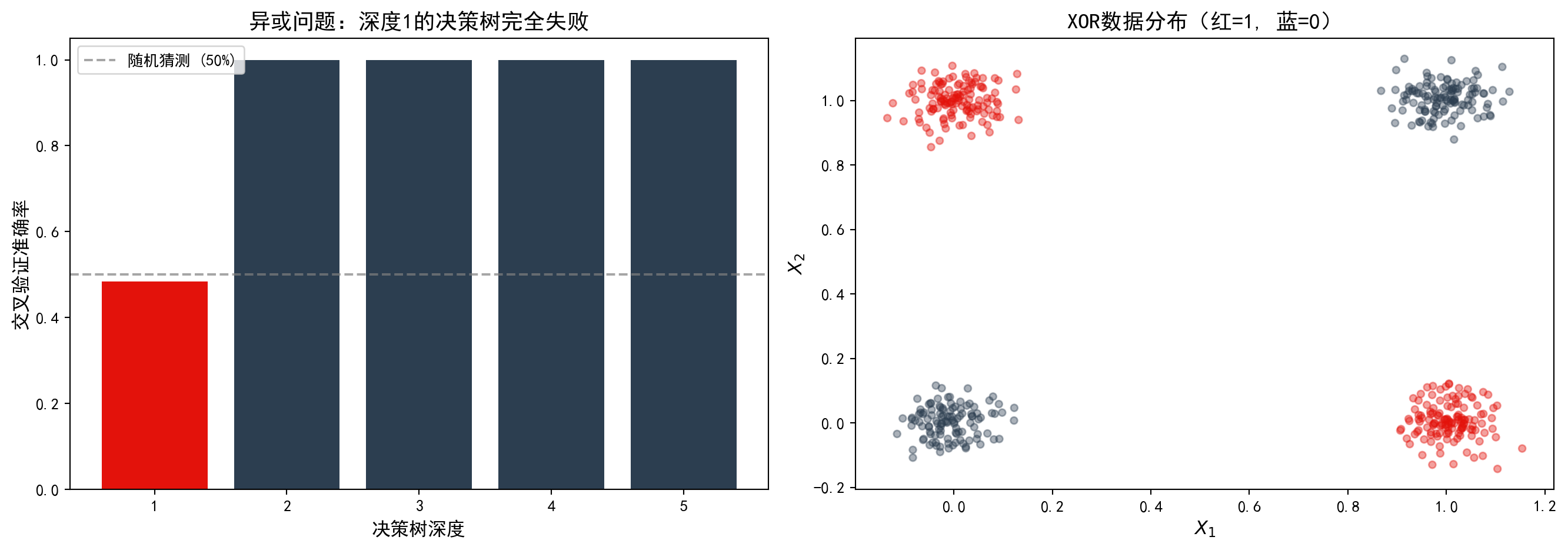
异或问题决策树可视化完成。下面输出不同深度的准确率对比与结论。
The XOR decision tree visualization is complete. Below we output the accuracy comparison across different depths along with conclusions.
print(f'深度=1准确率: {xor_accuracy_per_depth[0]:.4f}(≈随机猜测)')  # 输出深度=1的准确率
# Print accuracy at depth=1
print(f'深度=2准确率: {xor_accuracy_per_depth[1]:.4f}(完美解决XOR)')  # 输出深度=2的准确率
# Print accuracy at depth=2
print('结论: 单层切分无法捕捉交互效应,需要至少两层深度')  # 输出核心结论
# Print core conclusion
深度=1准确率: 0.4840(≈随机猜测)
深度=2准确率: 1.0000(完美解决XOR)
结论: 单层切分无法捕捉交互效应,需要至少两层深度上述代码的运行结果验证了理论预测:深度为1的决策桩(Decision Stump)准确率仅为 0.4840,与随机猜测(0.50)几乎无异;而深度为2的决策树准确率跃升至 1.0000,完美解决了异或问题。这一实验深刻揭示了贪心分裂策略的局限性——单次最优切分只能沿一个特征划分空间,完全无法捕捉 \(X_1\) 与 \(X_2\) 之间的交互效应。只有当树深度达到2层时,模型才能在第一层按 \(X_1\)(或 \(X_2\))分裂后,在第二层进一步按另一个特征分裂,从而构建出能识别”对角线”模式的决策边界。这也是为什么深度学习中的多层非线性变换比单层感知机更为强大的根本原因。
The results above confirm the theoretical prediction: a decision stump (depth 1) achieves an accuracy of only 0.4840, nearly indistinguishable from random guessing (0.50); whereas the depth-2 decision tree jumps to 1.0000, perfectly solving the XOR problem. This experiment profoundly reveals the limitation of the greedy splitting strategy — a single optimal split can only partition the space along one feature and is completely unable to capture the interaction effect between \(X_1\) and \(X_2\). Only when the tree depth reaches 2 can the model first split on \(X_1\) (or \(X_2\)) at the first level and then further split on the other feature at the second level, thereby constructing a decision boundary that recognizes the “diagonal” pattern. This is also the fundamental reason why multi-layer nonlinear transformations in deep learning are far more powerful than a single-layer perceptron.
2. 拟合噪声 (Fitting Noise) - 实验:生成一个完全随机的数据集(\(X\) 和 \(Y\) 都是乱码)。 - 操作:把决策树的深度设为 None(不限制)。 - 结果:你会惊讶地发现,训练集准确率竟然达到了 100%! - 解释:决策树”记忆”了每一个样本点。但这棵树在测试集上的表现会是灾难性的(随机猜测)。这就是过拟合的教科书案例。
2. Fitting Noise - Experiment: Generate a completely random dataset (both \(X\) and \(Y\) are noise). - Operation: Set the decision tree depth to None (no limit). - Result: You will be surprised to find that the training accuracy reaches 100%! - Explanation: The decision tree “memorized” every single data point. However, this tree’s performance on the test set will be disastrous (random guessing). This is a textbook case of overfitting.
如 图 12.7 所示,不限深度的决策树完美”记忆”了训练数据中的噪声。
As shown in 图 12.7, an unrestricted-depth decision tree perfectly “memorizes” the noise in the training data.
# ========== 导入所需库 ==========
# ========== Import Required Libraries ==========
import numpy as np  # 导入NumPy用于数值计算
# Import NumPy for numerical computation
import matplotlib.pyplot as plt  # 导入Matplotlib用于可视化
# Import Matplotlib for visualization
from sklearn.tree import DecisionTreeClassifier  # 导入决策树分类器
# Import decision tree classifier
from sklearn.model_selection import train_test_split  # 导入数据集划分函数
# Import train-test split function

# ========== 第1步:生成完全随机的噪声数据 ==========
# ========== Step 1: Generate Completely Random Noise Data ==========
np.random.seed(42)  # 设置随机种子确保结果可复现
# Set random seed for reproducibility
noise_sample_size = 200  # 样本量设为200
# Set sample size to 200
noise_feature_matrix = np.random.randn(noise_sample_size, 5)  # 生成5个完全随机的特征(标准正态分布)
# Generate 5 completely random features (standard normal distribution)
noise_target_variable = np.random.randint(0, 2, noise_sample_size)  # 生成完全随机的二分类标签(与X无关)
# Generate completely random binary labels (independent of X)

# ========== 第2步:划分训练集与测试集 ==========
# ========== Step 2: Split into Training and Test Sets ==========
noise_features_train, noise_features_test, noise_target_train, noise_target_test = train_test_split(  # 划分噪声数据的训练集与测试集
    # Split noise data into training and test sets
    noise_feature_matrix, noise_target_variable, test_size=0.3, random_state=42  # 70%训练,30%测试
    # 70% training, 30% testing
)

# ========== 第3步:遍历不同深度训练决策树并记录准确率 ==========
# ========== Step 3: Train Decision Trees at Various Depths and Record Accuracies ==========
noise_candidate_depths = list(range(1, 20)) + [None]  # 候选深度1~19加上无限深度(None)
# Candidate depths from 1 to 19 plus unlimited depth (None)
noise_training_accuracy_list = []  # 存储训练集准确率
# Store training set accuracies
noise_testing_accuracy_list = []  # 存储测试集准确率
# Store test set accuracies

for current_depth in noise_candidate_depths:  # 遍历每个候选深度
    # Iterate over each candidate depth
    noise_tree_model = DecisionTreeClassifier(max_depth=current_depth, random_state=42)  # 创建指定深度的决策树
    # Create a decision tree with the specified depth
    noise_tree_model.fit(noise_features_train, noise_target_train)  # 在训练集上拟合模型
    # Fit the model on the training set
    noise_training_accuracy_list.append(noise_tree_model.score(noise_features_train, noise_target_train))  # 记录训练集准确率
    # Record training set accuracy
    noise_testing_accuracy_list.append(noise_tree_model.score(noise_features_test, noise_target_test))  # 记录测试集准确率
    # Record test set accuracy
噪声数据生成和不同深度决策树的交叉验证完成。下面通过折线图可视化训练集与测试集准确率随深度变化的趋势。
Noise data generation and decision tree evaluation across different depths are complete. The following line chart visualizes how training and test set accuracies change with tree depth.
# ========== 第4步:可视化训练/测试准确率随深度变化趋势 ==========
# ========== Step 4: Visualize Training/Test Accuracy Trends Across Depths ==========
noise_figure, noise_axes = plt.subplots(figsize=(10, 6))  # 创建画布
# Create figure
depth_labels = [str(d) if d is not None else '∞' for d in noise_candidate_depths]  # 生成深度标签(None显示为∞)
# Generate depth labels (None displayed as ∞)
x_positions = range(len(noise_candidate_depths))  # 生成X轴位置序列
# Generate x-axis position sequence

noise_axes.plot(x_positions, noise_training_accuracy_list, 'o-', color='#E3120B', linewidth=2, label='训练集准确率')  # 绘制训练集曲线(红色)
# Plot training accuracy curve (red)
noise_axes.plot(x_positions, noise_testing_accuracy_list, 's-', color='#2C3E50', linewidth=2, label='测试集准确率')  # 绘制测试集曲线(深蓝)
# Plot test accuracy curve (dark blue)
noise_axes.axhline(y=0.5, color='gray', linestyle='--', alpha=0.7, label='随机猜测 (50%)')  # 添加50%基准线
# Add 50% random-guess baseline
noise_axes.set_xticks(x_positions)  # 设置X轴刻度位置
# Set x-axis tick positions
noise_axes.set_xticklabels(depth_labels, rotation=45)  # 设置X轴刻度标签并旋转45度
# Set x-axis tick labels and rotate 45 degrees
noise_axes.set_xlabel('决策树深度', fontsize=12)  # 设置X轴标签
# Set x-axis label
noise_axes.set_ylabel('准确率', fontsize=12)  # 设置Y轴标签
# Set y-axis label
noise_axes.set_title('纯噪声数据:训练准确率100% 但测试≈50%(过拟合)', fontsize=14)  # 设置图表标题
# Set chart title
noise_axes.legend()  # 显示图例
# Show legend
noise_axes.grid(True, alpha=0.3)  # 添加半透明网格线
# Add semi-transparent grid lines
plt.tight_layout()  # 自动调整布局
# Automatically adjust layout
plt.show()  # 展示图表
# Display the chart

# ========== 第5步:输出过拟合结论 ==========
# ========== Step 5: Output Overfitting Conclusions ==========
print(f'不限深度训练准确率: {noise_training_accuracy_list[-1]:.4f}')  # 输出无限深度时训练集准确率(应为100%)
# Print training accuracy at unlimited depth (should be 100%)
print(f'不限深度测试准确率: {noise_testing_accuracy_list[-1]:.4f}')  # 输出无限深度时测试集准确率(应约50%)
# Print test accuracy at unlimited depth (should be ~50%)
print('结论: 决策树"记忆"了每个样本点,但无法泛化到新数据')  # 输出过拟合核心结论
# Print core conclusion on overfitting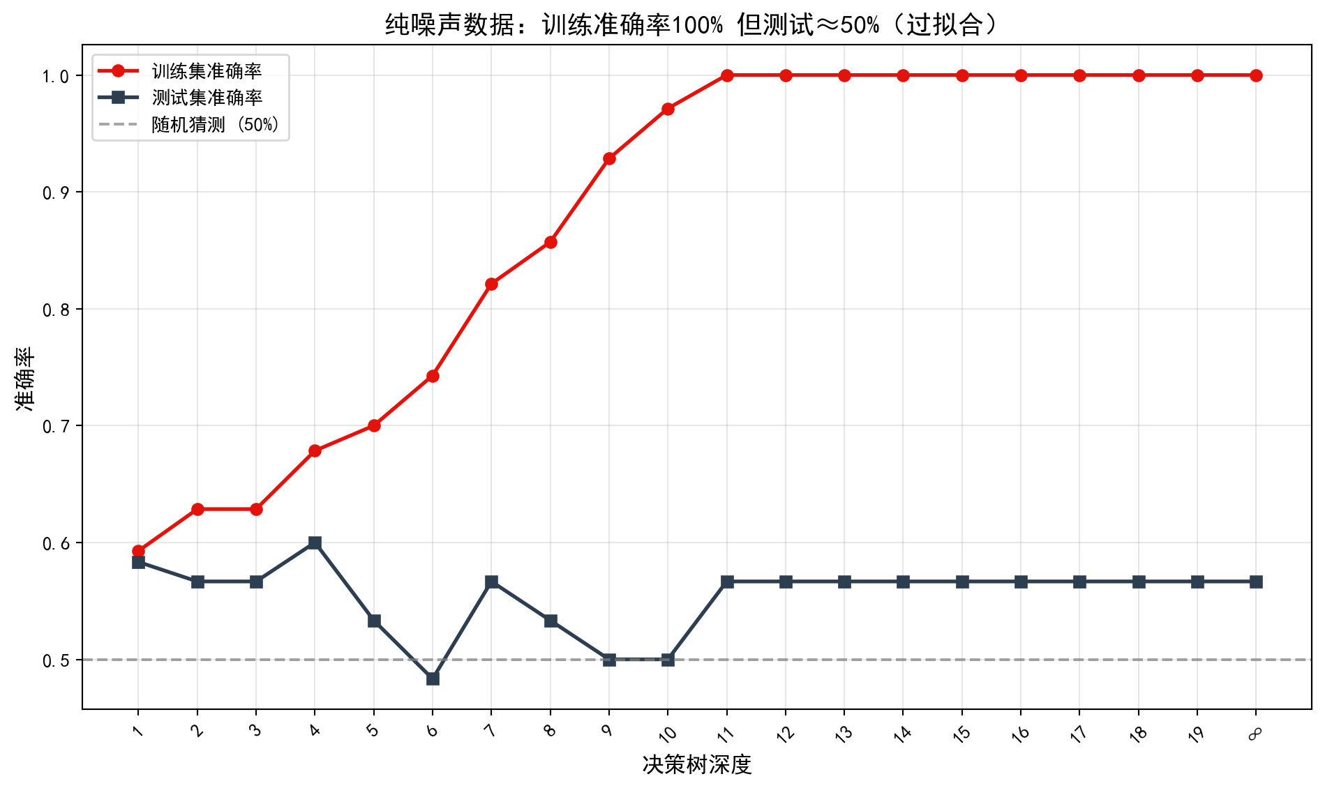
不限深度训练准确率: 1.0000
不限深度测试准确率: 0.5667
结论: 决策树"记忆"了每个样本点,但无法泛化到新数据
图 12.7 的运行结果和数值输出提供了过拟合的经典实证。在纯噪声数据(特征 \(X\) 与目标 \(Y\) 完全独立)上,不限深度的决策树训练集准确率高达 1.0000(100%),而测试集准确率仅为 0.5667,几乎等同于随机猜测(50%)。从图形来看,随着树深度增加,红色的训练集准确率曲线单调上升并最终达到100%,而深蓝色的测试集准确率曲线始终在50%的灰色虚线附近波动,两条曲线之间的”剪刀差”不断扩大。
The results and numerical output from 图 12.7 provide classic empirical evidence of overfitting. On pure noise data (where features \(X\) and target \(Y\) are completely independent), the unrestricted-depth decision tree achieves a training accuracy as high as 1.0000 (100%), while the test accuracy is only 0.5667, nearly equivalent to random guessing (50%). From the plot, as tree depth increases, the red training accuracy curve monotonically rises and eventually reaches 100%, while the dark blue test accuracy curve consistently fluctuates around the 50% gray dashed baseline, with the “scissors gap” between the two curves widening continuously.
这组结果深刻说明了一个核心原理:决策树的无限分裂能力使其可以”记忆”训练集中的每一个样本点——即使这些样本之间不存在任何真实的统计规律。在噪声数据中,每一次分裂都只是在拟合随机波动而非捕捉信号,因此模型的”知识”完全无法迁移到新数据上。这正是树深度限制、剪枝、以及集成方法(如随机森林、XGBoost)等正则化策略存在的根本原因——它们通过约束模型复杂度,强制模型放弃对噪声的记忆,从而提升泛化能力。
These results profoundly illustrate a core principle: the unlimited splitting capability of decision trees allows them to “memorize” every single data point in the training set — even when no genuine statistical pattern exists among these samples. In noise data, every split merely fits random fluctuations rather than capturing signals, so the model’s “knowledge” cannot transfer to new data at all. This is precisely the fundamental reason why regularization strategies such as depth limits, pruning, and ensemble methods (e.g., Random Forests, XGBoost) exist — they constrain model complexity, forcing the model to abandon its memorization of noise, thereby improving generalization ability. ## 习题与解答 (Exercises and Solutions) {#sec-exercises-ch12}
12.6.2 习题 (Problems)
习题1: 决策树分割准则
- 推导二分类问题中基尼不纯度的公式\(G(p) = 2p(1-p)\)
- 证明当\(p=0.5\)时基尼不纯度最大
- 比较基尼不纯度和熵在\(p \in [0,1]\)上的曲线
Exercise 1: Decision Tree Splitting Criteria
- Derive the Gini impurity formula \(G(p) = 2p(1-p)\) for a binary classification problem
- Prove that the Gini impurity is maximized when \(p=0.5\)
- Compare the curves of Gini impurity and entropy over \(p \in [0,1]\)
习题2: 随机森林调参
使用本地财务数据:
- 比较不同
n_estimators值(50, 100, 200, 500)对性能的影响 - 使用网格搜索调优
max_depth和min_samples_leaf - 分析OOB误差与测试误差的关系
Exercise 2: Random Forest Hyperparameter Tuning
Using local financial data:
- Compare the impact of different
n_estimatorsvalues (50, 100, 200, 500) on performance - Use grid search to tune
max_depthandmin_samples_leaf - Analyze the relationship between OOB error and test error
习题3: Boosting vs Bagging
- 解释Bagging和Boosting在方差-偏差权衡上的区别
- 在同一数据集上比较随机森林和XGBoost的性能
- 讨论何时使用哪种方法
Exercise 3: Boosting vs Bagging
- Explain the differences between Bagging and Boosting in terms of the bias-variance tradeoff
- Compare the performance of Random Forest and XGBoost on the same dataset
- Discuss when to use which method
习题4: 特征重要性分析
- 比较基于Gini的重要性和Permutation重要性
- 使用SHAP分析单个样本的预测
- 讨论特征重要性的局限性
Exercise 4: Feature Importance Analysis
- Compare Gini-based importance and Permutation importance
- Use SHAP to analyze the prediction for a single observation
- Discuss the limitations of feature importance
12.6.3 解答 (Solutions)
习题1解答
Solution to Exercise 1
import numpy as np  # 导入数值计算库
# Import numerical computation library
import matplotlib.pyplot as plt  # 导入绘图库
# Import plotting library

# ========== 第1步:输出基尼不纯度的数学推导 ==========
# ========== Step 1: Output the mathematical derivation of Gini impurity ==========
print('=== 习题1解答: 决策树分割准则 ===\n')  # 打印解答标题
# Print the solution header

print('(a) 基尼不纯度推导:')  # 输出第(a)小题解答
# Output the answer for part (a)
print('''
对于二分类问题,设类别1的比例为p,类别0的比例为1-p

基尼不纯度定义:
G = ∑_{k} p_k(1-p_k)
  = p(1-p) + (1-p)(1-(1-p))
  = p(1-p) + (1-p)p
  = 2p(1-p)  ✓
''')  # 展示基尼不纯度公式的完整推导过程
# Display the complete derivation of the Gini impurity formula
=== 习题1解答: 决策树分割准则 ===
(a) 基尼不纯度推导:
对于二分类问题,设类别1的比例为p,类别0的比例为1-p
基尼不纯度定义:
G = ∑_{k} p_k(1-p_k)
= p(1-p) + (1-p)(1-(1-p))
= p(1-p) + (1-p)p
= 2p(1-p) ✓
基尼不纯度公式推导完毕。下面证明其在p=0.5处取得最大值。
The derivation of the Gini impurity formula is complete. Next, we prove that it attains its maximum at p=0.5.
# ========== 第2步:证明基尼不纯度在p=0.5时取最大值 ==========
# ========== Step 2: Prove that Gini impurity is maximized at p=0.5 ==========
print('(b) 最大值证明:')  # 输出第(b)小题解答
# Output the answer for part (b)
print('''
对G(p) = 2p(1-p) = 2p - 2p²求导:
dG/dp = 2 - 4p = 0
解得 p = 0.5

二阶导数: d²G/dp² = -4 < 0
因此 p = 0.5 是最大值点

G(0.5) = 2 × 0.5 × 0.5 = 0.5  ✓
''')  # 展示求导、二阶导判定的完整证明过程
# Display the complete proof using first and second derivative tests
(b) 最大值证明:
对G(p) = 2p(1-p) = 2p - 2p²求导:
dG/dp = 2 - 4p = 0
解得 p = 0.5
二阶导数: d²G/dp² = -4 < 0
因此 p = 0.5 是最大值点
G(0.5) = 2 × 0.5 × 0.5 = 0.5 ✓
基尼不纯度的推导和最大值证明完毕。下面通过可视化对比基尼不纯度函数和信息熵函数的形态差异。
The derivation and maximum value proof for Gini impurity are complete. Next, we visually compare the shapes of the Gini impurity function and the entropy function.
# ========== 第3步:可视化比较基尼不纯度与熵 ==========
# ========== Step 3: Visually compare Gini impurity and entropy ==========
p = np.linspace(0.001, 0.999, 100)  # 生成p从0.001到0.999的100个等距点
# Generate 100 equally spaced points for p from 0.001 to 0.999
gini = 2 * p * (1 - p)  # 计算基尼不纯度 G(p) = 2p(1-p)
# Compute Gini impurity G(p) = 2p(1-p)
entropy = -p * np.log2(p) - (1-p) * np.log2(1-p)  # 计算信息熵 H(p) = -plog2(p) - (1-p)log2(1-p)
# Compute entropy H(p) = -p log2(p) - (1-p) log2(1-p)

plt.figure(figsize=(10, 6))  # 创建画布
# Create the figure canvas
plt.plot(p, gini, 'r-', linewidth=2, label='基尼不纯度: 2p(1-p)')  # 绘制基尼曲线(红色)
# Plot the Gini curve (red)
plt.plot(p, entropy, 'b-', linewidth=2, label='熵: -p log₂p - (1-p)log₂(1-p)')  # 绘制熵曲线(蓝色)
# Plot the entropy curve (blue)
plt.xlabel('类别1的比例 p', fontsize=12)  # 设置X轴标签
# Set the X-axis label
plt.ylabel('不纯度度量', fontsize=12)  # 设置Y轴标签
# Set the Y-axis label
plt.title('基尼不纯度 vs 熵', fontsize=14)  # 设置图表标题
# Set the chart title
plt.legend()  # 显示图例
# Display the legend
plt.grid(True, alpha=0.3)  # 添加半透明网格线
# Add semi-transparent grid lines
plt.axvline(x=0.5, color='gray', linestyle='--', alpha=0.5)  # 在p=0.5处添加端线
# Add a dashed vertical line at p=0.5
plt.tight_layout()  # 自动调整布局
# Automatically adjust the layout
plt.show()  # 展示图表
# Display the chart

# ========== 第4步:输出观察结论 ==========
# ========== Step 4: Output the observational conclusions ==========
print('(c) 观察: 两条曲线形状相似,都在p=0.5处达到最大值')  # 输出相似性观察
# Print the similarity observation
print('    熵的值域[0,1],基尼的值域[0,0.5]')  # 输出值域差异
# Print the range difference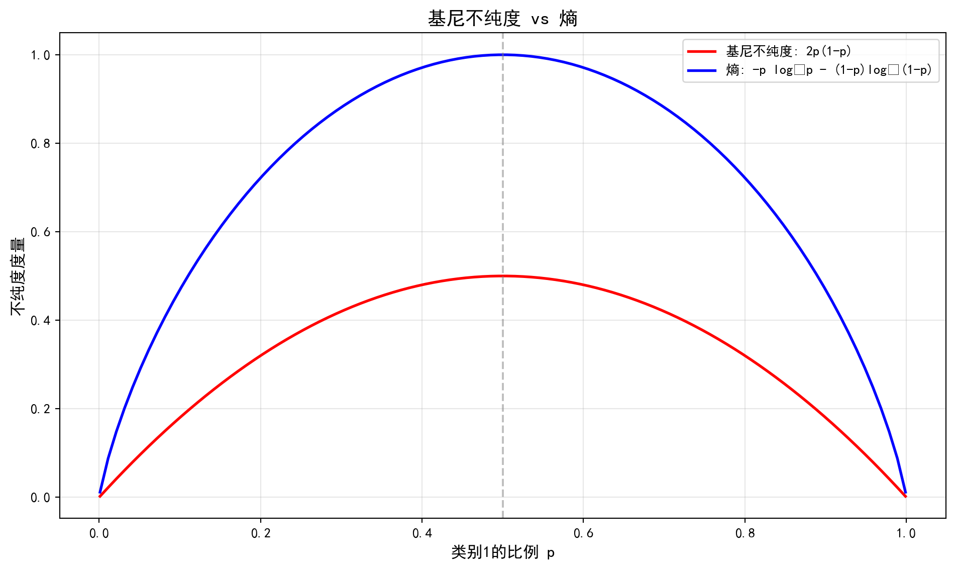
(c) 观察: 两条曲线形状相似,都在p=0.5处达到最大值
    熵的值域[0,1],基尼的值域[0,0.5]
习题2解答
Solution to Exercise 2
# ========== 导入所需库 ==========
# ========== Import required libraries ==========
from sklearn.ensemble import RandomForestClassifier  # 导入随机森林分类器
# Import the Random Forest classifier
from sklearn.model_selection import cross_val_score, GridSearchCV  # 导入交叉验证和网格搜索
# Import cross-validation and grid search

print('=== 习题2解答: 随机森林调参 ===\n')  # 打印解答标题
# Print the solution header

# ========== 第1步:比较不同n_estimators对模型性能的影响 ==========
# ========== Step 1: Compare the impact of different n_estimators on model performance ==========
print('(a) n_estimators影响:')  # 输出第(a)小题标题
# Output the title for part (a)
candidate_n_estimators_list = [50, 100, 200, 500]  # 候选的树数量列表
# List of candidate numbers of trees
n_estimators_evaluation_results_list = []  # 存储评估结果
# Store evaluation results

for current_n_estimators in candidate_n_estimators_list:  # 遍历每个候选树数量
    # Iterate over each candidate number of trees
    temporary_random_forest_model = RandomForestClassifier(  # 创建随机森林模型
        # Create a Random Forest model
        n_estimators=current_n_estimators,  # 设置当前树数量
        # Set the current number of trees
        max_depth=6,  # 固定最大深度为6
        # Fix the maximum depth at 6
        class_weight='balanced',  # 设置类别权重平衡
        # Set balanced class weights
        random_state=42,  # 固定随机种子
        # Fix the random seed
        n_jobs=-1  # 使用所有CPU核心并行计算
        # Use all CPU cores for parallel computation
    )
    temporary_cross_validation_scores = cross_val_score(temporary_random_forest_model, features_train_matrix, target_train_series, cv=5, scoring='roc_auc')  # 5折交叉验证评估AUC
    # Evaluate AUC using 5-fold cross-validation
    n_estimators_evaluation_results_list.append({  # 记录评估结果
        # Record the evaluation results
        'n_estimators': current_n_estimators,  # 树数量
        # Number of trees
        'CV_AUC_mean': temporary_cross_validation_scores.mean(),  # 平均AUC
        # Mean AUC
        'CV_AUC_std': temporary_cross_validation_scores.std()  # AUC标准差
        # AUC standard deviation
    })
    print(f'n_estimators={current_n_estimators}: AUC={temporary_cross_validation_scores.mean():.4f} ± {temporary_cross_validation_scores.std():.4f}')  # 输出每个配置的AUC结果
    # Output the AUC result for each configuration
=== 习题2解答: 随机森林调参 ===
(a) n_estimators影响:
n_estimators=50: AUC=0.7703 ± 0.0384
n_estimators=100: AUC=0.7702 ± 0.0436
n_estimators=200: AUC=0.7691 ± 0.0490
n_estimators=500: AUC=0.7750 ± 0.0544n_estimators影响评估完成。下面通过网格搜索调优超参数并分析OOB误差。
The evaluation of the n_estimators impact is complete. Next, we tune hyperparameters via grid search and analyze OOB error.
# ========== 第2步:网格搜索调优max_depth和min_samples_leaf ==========
# ========== Step 2: Grid search to tune max_depth and min_samples_leaf ==========
print('\n(b) 网格搜索调优:')  # 输出第(b)小题标题
# Output the title for part (b)
hyperparameter_search_grid = {  # 定义超参数搜索空间
    # Define the hyperparameter search space
    'max_depth': [4, 6, 8],  # 候选最大深度
    # Candidate maximum depths
    'min_samples_leaf': [10, 20, 30]  # 候选最小叶节点样本数
    # Candidate minimum samples per leaf
}

# 为节省计算时间,使用100棵树(实际生产环境建议使用500棵以上)
# To save computation time, use 100 trees (500+ recommended for production)
random_forest_grid_search_model = GridSearchCV(  # 创建网格搜索对象
    # Create the grid search object
    RandomForestClassifier(n_estimators=100, class_weight='balanced',  # 基础随机森林配置
        # Base Random Forest configuration
                          random_state=42, n_jobs=-1),  # 固定随机种子
        # Fix the random seed
    hyperparameter_search_grid,  # 传入搜索空间
    # Pass in the search space
    cv=3,  # 3折交叉验证
    # 3-fold cross-validation
    scoring='roc_auc',  # 以AUC为评估指标
    # Use AUC as the evaluation metric
    n_jobs=-1  # 并行计算
    # Parallel computation
)
random_forest_grid_search_model.fit(features_train_matrix, target_train_series)  # 执行网格搜索
# Execute the grid search

print(f'最优参数: {random_forest_grid_search_model.best_params_}')  # 输出网格搜索找到的最优参数组合
# Output the best parameter combination found by grid search
print(f'最优CV AUC: {random_forest_grid_search_model.best_score_:.4f}')  # 输出最优交叉验证AUC
# Output the best cross-validation AUC
(b) 网格搜索调优:
最优参数: {'max_depth': 4, 'min_samples_leaf': 30}
最优CV AUC: 0.7952
网格搜索调优完毕。下面分析袋外(OOB)误差与测试误差的关系。
Grid search tuning is complete. Next, we analyze the relationship between Out-of-Bag (OOB) error and test error.
# ========== 第3步:分析OOB误差与测试误差的关系 ==========
# ========== Step 3: Analyze the relationship between OOB error and test error ==========
print('\n(c) OOB误差分析:')  # 输出第(c)小题标题
# Output the title for part (c)
out_of_bag_random_forest_model = RandomForestClassifier(  # 创建带OOB评估的随机森林
    # Create a Random Forest with OOB evaluation enabled
    **random_forest_grid_search_model.best_params_,  # 使用网格搜索找到的最优参数
    # Use the best parameters found by grid search
    n_estimators=200,  # 200棵树
    # 200 trees
    class_weight='balanced',  # 类别权重平衡
    # Balanced class weights
    oob_score=True,  # 启用袋外(Out-of-Bag)评估
    # Enable Out-of-Bag evaluation
    random_state=42,  # 固定随机种子
    # Fix the random seed
    n_jobs=-1  # 并行计算
    # Parallel computation
)
out_of_bag_random_forest_model.fit(features_train_matrix, target_train_series)  # 在训练集上拟合模型
# Fit the model on the training set
out_of_bag_test_score = out_of_bag_random_forest_model.score(features_test_matrix, target_test_series)  # 计算测试集准确率
# Compute the test set accuracy

print(f'OOB得分: {out_of_bag_random_forest_model.oob_score_:.4f}')  # 输出袋外评估得分
# Output the OOB evaluation score
print(f'测试集得分: {out_of_bag_test_score:.4f}')  # 输出测试集得分
# Output the test set score
print('OOB是测试误差的良好近似,无需单独的验证集')  # 输出OOB评估的核心结论
# Output the key conclusion: OOB is a good approximation of test error, no separate validation set needed
(c) OOB误差分析:
OOB得分: 0.8404
测试集得分: 0.8587
OOB是测试误差的良好近似,无需单独的验证集
习题3解答
Solution to Exercise 3
# ========== 第1步:输出方差-偏差权衡的理论分析 ==========
# ========== Step 1: Output the theoretical analysis of the bias-variance tradeoff ==========
print('=== 习题3解答: Boosting vs Bagging ===\n')  # 打印解答标题
# Print the solution header

print('(a) 方差-偏差权衡:')  # 输出第(a)小题标题
# Output the title for part (a)
print('''
Bagging (随机森林):
- 主要降低方差
- 基模型可以较复杂(高方差)
- 通过平均多个模型减少方差
- 偏差基本不变

Boosting (XGBoost):
- 同时降低偏差和方差
- 基模型通常较简单(高偏差,浅树)
- 通过串行纠错减少偏差
- 但过多迭代可能增加方差(过拟合)
''')  # 输出Bagging与Boosting的理论对比
# Output the theoretical comparison between Bagging and Boosting
=== 习题3解答: Boosting vs Bagging ===
(a) 方差-偏差权衡:
Bagging (随机森林):
- 主要降低方差
- 基模型可以较复杂(高方差)
- 通过平均多个模型减少方差
- 偏差基本不变
Boosting (XGBoost):
- 同时降低偏差和方差
- 基模型通常较简单(高偏差,浅树)
- 通过串行纠错减少偏差
- 但过多迭代可能增加方差(过拟合)
Boosting与Bagging的理论对比输出完毕。下面在真实数据上比较两种方法的实际表现。
The theoretical comparison between Boosting and Bagging is complete. Next, we compare the actual performance of both methods on real data.
# ========== 第2步:在真实财务风险数据上比较模型性能 ==========
# ========== Step 2: Compare model performance on real financial risk data ==========
print('(b) 在财务风险数据上的比较:')  # 输出第(b)小题标题
# Output the title for part (b)
print(f'随机森林测试AUC: {roc_auc_score(target_test_series, random_forest_predicted_probabilities):.4f}')  # 输出随机森林测试AUC
# Output the Random Forest test AUC
print(f'XGBoost测试AUC: {roc_auc_score(target_test_series, xgboost_predicted_probabilities_array):.4f}')  # 输出XGBoost测试AUC
# Output the XGBoost test AUC

# ========== 第3步:输出方法选择建议 ==========
# ========== Step 3: Output method selection recommendations ==========
print('\n(c) 方法选择建议:')  # 输出第(c)小题标题
# Output the title for part (c)
print('''
选择随机森林:
- 数据噪声大
- 需要稳健预测
- 计算资源有限
- 需要OOB估计

选择XGBoost:
- 追求最高预测精度
- 有足够调参时间
- 数据相对干净
- Kaggle竞赛场景
''')  # 输出两种方法的适用场景建议
# Output the recommended use cases for both methods
(b) 在财务风险数据上的比较:
随机森林测试AUC: 0.8414
XGBoost测试AUC: 0.8247
(c) 方法选择建议:
选择随机森林:
- 数据噪声大
- 需要稳健预测
- 计算资源有限
- 需要OOB估计
选择XGBoost:
- 追求最高预测精度
- 有足够调参时间
- 数据相对干净
- Kaggle竞赛场景
习题4解答
Solution to Exercise 4
# ========== 导入所需库 ==========
# ========== Import required libraries ==========
from sklearn.inspection import permutation_importance  # 导入置换重要性计算函数
# Import the permutation importance computation function

print('=== 习题4解答: 特征重要性分析 ===\n')  # 打印解答标题
# Print the solution header

# ========== 第1步:计算并对比两种特征重要性方法 ==========
# ========== Step 1: Compute and compare two feature importance methods ==========
print('(a) 基于Gini vs Permutation重要性:')  # 输出第(a)小题标题
# Output the title for part (a)

gini_feature_importance_array = fitted_random_forest_classifier.feature_importances_  # 获取基于Gini不纯度下降的特征重要性
# Retrieve feature importance based on Gini impurity reduction

# 计算基于置换的特征重要性(打乱某特征后观察模型性能下降幅度)
# Compute permutation-based feature importance (observe model performance drop after shuffling a feature)
permutation_importance_result_object = permutation_importance(fitted_random_forest_classifier, features_test_matrix, target_test_series,  # 计算置换特征重要性
    # Compute permutation feature importance
                                     n_repeats=10, random_state=42, n_jobs=-1)  # 重复10次置换实验
    # Repeat the permutation experiment 10 times
permutation_feature_importance_array = permutation_importance_result_object.importances_mean  # 提取置换重要性均值
# Extract the mean permutation importance values

# ========== 第2步:输出两种重要性的对比表 ==========
# ========== Step 2: Output the comparison table of both importance measures ==========
importance_comparison_dataframe = pd.DataFrame({  # 创建对比表格
    # Create the comparison table
    '特征': predictor_variables_list,  # 特征名称列
    # Feature name column
    'Gini重要性': gini_feature_importance_array,  # Gini方法的重要性值
    # Importance values from the Gini method
    'Permutation重要性': permutation_feature_importance_array  # 置换方法的重要性值
    # Importance values from the Permutation method
})
print(importance_comparison_dataframe.round(4).to_string(index=False))  # 输出保留4位小数的对比表
# Output the comparison table rounded to 4 decimal places
=== 习题4解答: 特征重要性分析 ===
(a) 基于Gini vs Permutation重要性:
特征 Gini重要性 Permutation重要性
roa 0.4950 0.0190
debt_ratio 0.1331 0.0002
current_ratio 0.2006 -0.0097
log_assets 0.1713 0.0057两种特征重要性度量对比表输出完毕。下面分析两种方法的优劣并总结特征重要性的局限性。
The comparison table of the two feature importance measures is complete. Next, we analyze the pros and cons of both methods and summarize the limitations of feature importance.
# ========== 第3步:输出两种方法的对比分析 ==========
# ========== Step 3: Output the comparative analysis of both methods ==========
print('\n比较:')  # 输出比较标题
# Print the comparison header
print('- Gini重要性: 基于树分裂时的不纯度减少,可能偏向高基数特征')  # 解释Gini方法的特点与局限
# Explain the characteristics and limitations of the Gini method
print('- Permutation重要性: 打乱特征后性能下降,更可靠但计算量大')  # 解释Perm方法的特点与局限
# Explain the characteristics and limitations of the Permutation method

print('\n(b) SHAP单样本分析: 见SHAP特征重要性图')  # 指引读者参考SHAP部分
# Direct readers to the SHAP feature importance figure

# ========== 第4步:输出特征重要性方法的局限性总结 ==========
# ========== Step 4: Output the summary of limitations of feature importance methods ==========
print('\n(c) 特征重要性的局限性:')  # 输出第(c)小题标题
# Output the title for part (c)
print('''
1. 相关特征问题: 相关特征会"分享"重要性
2. 尺度敏感: 某些方法对特征尺度敏感
3. 不表示因果关系: 重要≠有因果效应
4. 交互效应: 无法捕捉特征间的交互
5. 样本外稳定性: 不同样本可能给出不同排序
''')  # 输出5条特征重要性方法的常见局限性
# Output 5 common limitations of feature importance methods
比较:
- Gini重要性: 基于树分裂时的不纯度减少,可能偏向高基数特征
- Permutation重要性: 打乱特征后性能下降,更可靠但计算量大

(b) SHAP单样本分析: 见SHAP特征重要性图

(c) 特征重要性的局限性:

1. 相关特征问题: 相关特征会"分享"重要性
2. 尺度敏感: 某些方法对特征尺度敏感
3. 不表示因果关系: 重要≠有因果效应
4. 交互效应: 无法捕捉特征间的交互
5. 样本外稳定性: 不同样本可能给出不同排序
12.7 本章小结 (Chapter Summary)
本章系统介绍了基于树的机器学习方法在中国资本市场中的应用。从单棵决策树的CART算法出发,我们依次讨论了分类树与回归树的分割准则(基尼不纯度与均方误差),并通过代价复杂度剪枝和交叉验证解决了过拟合问题。在此基础上,我们引入了随机森林(Bagging + 特征随机化)和XGBoost(梯度提升 + 正则化)两种集成方法,通过长三角上市公司的财务风险预测案例验证了集成方法在预测精度和稳定性上的显著优势。最后,我们探讨了SHAP值等模型可解释性工具,强调了在追求预测精度的同时保持模型透明度的重要性。树方法的核心启示是:单棵树易于理解但不稳定,集成方法通过”群体智慧”显著提升性能,而可解释性工具则为”黑盒”模型提供了打开透明之窗的钥匙。
This chapter systematically introduced the application of tree-based machine learning methods in the Chinese capital market. Starting from the CART algorithm for individual decision trees, we discussed the splitting criteria for classification trees and regression trees (Gini impurity and mean squared error), and addressed the overfitting problem through cost-complexity pruning and cross-validation. Building upon this foundation, we introduced two ensemble methods—Random Forest (Bagging + feature randomization) and XGBoost (gradient boosting + regularization)—and validated the significant advantages of ensemble methods in prediction accuracy and stability through a financial risk prediction case study of Yangtze River Delta listed companies. Finally, we explored model interpretability tools such as SHAP values, emphasizing the importance of maintaining model transparency while pursuing predictive accuracy. The core insight from tree methods is: A single tree is easy to understand but unstable; ensemble methods significantly improve performance through “collective wisdom”; and interpretability tools provide the key to opening a window of transparency into “black box” models.