11 广义线性模型与非线性模型 (Generalized Linear Models and Nonlinear Models)

当因变量不满足正态分布假设,或变量关系非线性时,需要使用广义线性模型(Generalized Linear Models, GLM)或其他非线性模型。本章系统介绍GLM的理论框架,重点讲解Logistic回归和Poisson回归,并介绍正则化方法。

When the dependent variable does not satisfy the normality assumption, or the relationship between variables is nonlinear, Generalized Linear Models (GLM) or other nonlinear models are needed. This chapter systematically introduces the theoretical framework of GLM, with a focus on Logistic regression and Poisson regression, and also covers regularization methods.

11.1 非线性模型在金融风险管理中的典型应用 (Typical Applications of Nonlinear Models in Financial Risk Management)

经典线性回归要求因变量服从正态分布，但金融领域中许多关键问题的因变量本质上是非正态的。GLM和非线性模型为解决这些问题提供了强大的工具。

Classical linear regression requires the dependent variable to follow a normal distribution, but in the field of finance, the dependent variables of many key problems are inherently non-normal. GLM and nonlinear models provide powerful tools for addressing these problems.

11.1.1 应用一：信用违约预测与Logistic回归 (Application 1: Credit Default Prediction and Logistic Regression)

信用风险管理的核心问题是预测借款人是否会违约——这是一个二分类问题，因变量只取0或1。经典线性回归会预测出超出[0,1]范围的概率值，且残差不满足正态性假设。Logistic回归通过logit连接函数完美解决了这一问题。利用 financial_statement.h5 中的财务比率（如资产负债率、流动比率、利息保障倍数等）作为自变量，以上市公司是否被ST标记作为违约代理变量，可以构建信用评分模型。

The core problem of credit risk management is predicting whether a borrower will default — this is a binary classification problem where the dependent variable takes only 0 or 1. Classical linear regression may predict probability values outside the [0,1] range, and the residuals do not satisfy the normality assumption. Logistic regression perfectly solves this problem through the logit link function. Using financial ratios from financial_statement.h5 (such as debt-to-asset ratio, current ratio, interest coverage ratio, etc.) as independent variables, and whether a listed company is marked as ST as a proxy variable for default, a credit scoring model can be constructed.

11.1.2 应用二：金融事件计数的Poisson回归 (Application 2: Poisson Regression for Financial Event Counts)

上市公司每季度发布公告的次数、分析师发布研究报告的次数、股票涨停或跌停的天数——这些都是计数变量。Poisson回归假设因变量服从泊松分布，通过对数连接函数将均值与线性预测量联系起来。基于 financial_statement.h5 和 stock_price_pre_adjusted.h5 的数据，可以研究公司特征（如规模、行业、治理质量）与异常事件发生频率之间的关系。

The number of announcements released by listed companies each quarter, the number of research reports published by analysts, and the number of days a stock hits its price limit up or down — these are all count variables. Poisson regression assumes the dependent variable follows a Poisson distribution and links the mean to the linear predictor through a log link function. Based on data from financial_statement.h5 and stock_price_pre_adjusted.h5, one can study the relationship between company characteristics (such as size, industry, governance quality) and the frequency of abnormal events.

11.1.3 应用三：正则化与高维金融数据 (Application 3: Regularization and High-Dimensional Financial Data)

当模型中引入大量候选变量时（如 valuation_factors_quarterly_15_years.h5 中包含众多估值因子），模型面临过拟合和多重共线性风险。LASSO和Ridge等正则化方法通过向目标函数中添加惩罚项，在拟合数据和模型复杂度之间取得平衡。在A股市场的多因子选股研究中，正则化Logistic回归被广泛用于从数百个候选因子中筛选出真正有预测能力的关键因子。

When a large number of candidate variables are introduced into the model (such as the numerous valuation factors in valuation_factors_quarterly_15_years.h5), the model faces risks of overfitting and multicollinearity. Regularization methods such as LASSO and Ridge achieve a balance between fitting the data and model complexity by adding penalty terms to the objective function. In multi-factor stock selection research on the A-share market, regularized Logistic regression is widely used to screen out truly predictive key factors from hundreds of candidates.

11.2 指数族分布 (Exponential Family Distributions)

GLM要求因变量服从指数族分布(Exponential Family),其概率密度函数如式 11.1 所示:

GLM requires the dependent variable to follow an exponential family distribution, whose probability density function is shown in 式 11.1:

\[ f(y|\theta, \phi) = \exp\left\{\frac{y\theta - b(\theta)}{a(\phi)} + c(y, \phi)\right\} \tag{11.1}\]

其中:

\(\theta\): 自然参数(canonical parameter)
\(\phi\): 离散参数(dispersion parameter)
\(a(\cdot), b(\cdot), c(\cdot)\): 特定于分布的已知函数

Where:

\(\theta\): canonical parameter
\(\phi\): dispersion parameter
\(a(\cdot), b(\cdot), c(\cdot)\): known functions specific to the distribution

常见分布的指数族形式

Exponential Family Forms of Common Distributions

分布	\(\theta\)	\(b(\theta)\)	\(a(\phi)\)	均值 \(\mu\)	方差
正态	\(\mu\)	\(\theta^2/2\)	\(\sigma^2\)	\(\theta\)	\(\sigma^2\)
二项	\(\ln\frac{p}{1-p}\)	\(\ln(1+e^\theta)\)	\(1/n\)	\(\frac{e^\theta}{1+e^\theta}\)	\(np(1-p)\)
泊松	\(\ln\lambda\)	\(e^\theta\)	\(1\)	\(e^\theta\)	\(\lambda\)
伽马	\(-1/\mu\)	\(-\ln(-\theta)\)	\(\phi\)	\(-1/\theta\)	\(\phi\mu^2\)

指数族分布有重要性质:\(E(Y) = b'(\theta)\),\(\text{Var}(Y) = a(\phi)b''(\theta)\)

Exponential family distributions have important properties: \(E(Y) = b'(\theta)\), \(\text{Var}(Y) = a(\phi)b''(\theta)\)

11.3 广义线性模型(GLM)框架 (Generalized Linear Model (GLM) Framework)

11.3.1 模型的三要素 (Three Components of the Model)

GLM由三个相互关联的要素组成:

GLM consists of three interrelated components:

1. 随机分量(Random Component)

1. Random Component

因变量\(Y\)服从指数族分布,其均值为\(\mu = E(Y)\)。

The dependent variable \(Y\) follows an exponential family distribution with mean \(\mu = E(Y)\).

2. 系统分量(Systematic Component)

2. Systematic Component

线性预测子(Linear Predictor),如式 11.2 所示:

The linear predictor, as shown in 式 11.2:

\[ \eta = \mathbf{X}\boldsymbol{\beta} = \beta_0 + \beta_1 X_1 + ... + \beta_p X_p \tag{11.2}\]

3. 连接函数(Link Function)

3. Link Function

连接函数\(g(\cdot)\)将均值\(\mu\)与线性预测子\(\eta\)联系起来,如式 11.3 所示:

The link function \(g(\cdot)\) connects the mean \(\mu\) to the linear predictor \(\eta\), as shown in 式 11.3:

\[ g(\mu) = \eta \tag{11.3}\]

等价地:\(\mu = g^{-1}(\eta)\)

Equivalently: \(\mu = g^{-1}(\eta)\)

11.3.2 常用连接函数 (Common Link Functions)

表 11.1 列出了GLM中常用的连接函数及其应用场景。

表 11.1 lists the commonly used link functions in GLM and their application scenarios.

表 11.1: GLM常用连接函数

分布	典型连接函数	表达式	应用场景
正态	恒等(Identity)	\(g(\mu) = \mu\)	连续因变量
二项	Logit	\(g(\mu) = \ln\frac{\mu}{1-\mu}\)	二分类、比例
二项	Probit	\(g(\mu) = \Phi^{-1}(\mu)\)	二分类(潜变量)
泊松	对数(Log)	\(g(\mu) = \ln\mu\)	计数数据
伽马	倒数(Inverse)	\(g(\mu) = 1/\mu\)	正偏态连续变量

为什么需要连接函数？（直观理解）

Why Do We Need Link Functions? (Intuitive Understanding)

线性预测子 \(\eta = \mathbf{X}\boldsymbol{\beta}\) 的取值范围是 \((-\infty, +\infty)\)。但我们的因变量均值 \(\mu\) 往往有范围限制：

The range of the linear predictor \(\eta = \mathbf{X}\boldsymbol{\beta}\) is \((-\infty, +\infty)\). However, the mean of our dependent variable \(\mu\) often has range restrictions:

二分类概率 \(p \in [0, 1]\)
计数 \(\lambda \in [0, +\infty)\)
Binary classification probability \(p \in [0, 1]\)
Count \(\lambda \in [0, +\infty)\)

直接用线性回归（\(p = \mathbf{X}\boldsymbol{\beta}\)）可能会预测出负概率或大于1的概率，这是荒谬的。 连接函数 \(g(\cdot)\) 的作用就是进行空间映射：

Directly using linear regression (\(p = \mathbf{X}\boldsymbol{\beta}\)) may predict negative probabilities or probabilities greater than 1, which is absurd. The role of the link function \(g(\cdot)\) is to perform space mapping:

Logit将 \((0, 1)\) 映射到 \((-\infty, +\infty)\)
Log将 \((0, +\infty)\) 映射到 \((-\infty, +\infty)\)
Logit maps \((0, 1)\) to \((-\infty, +\infty)\)
Log maps \((0, +\infty)\) to \((-\infty, +\infty)\)

反过来，反连接函数 \(g^{-1}\) 将线性预测值”压缩”回合理的取值范围。这就是GLM”广义”的精髓所在。

Conversely, the inverse link function \(g^{-1}\) “compresses” the linear predicted values back into a reasonable range. This is the essence of the “generalized” in GLM.

11.3.3 极大似然估计 (Maximum Likelihood Estimation)

GLM参数通过极大似然估计(MLE)获得。对数似然函数如式 11.4 所示:

GLM parameters are obtained through Maximum Likelihood Estimation (MLE). The log-likelihood function is shown in 式 11.4:

\[ \ell(\boldsymbol{\beta}) = \sum_{i=1}^n \frac{y_i\theta_i - b(\theta_i)}{a(\phi)} + c(y_i, \phi) \tag{11.4}\]

由于\(\theta_i\)通过连接函数与\(\boldsymbol{\beta}\)相关,对数似然非线性于\(\boldsymbol{\beta}\),需要使用Newton-Raphson或Fisher Scoring迭代算法求解。

Since \(\theta_i\) is related to \(\boldsymbol{\beta}\) through the link function, the log-likelihood is nonlinear in \(\boldsymbol{\beta}\), requiring iterative algorithms such as Newton-Raphson or Fisher Scoring to solve.

迭代加权最小二乘(IRLS)

Iteratively Reweighted Least Squares (IRLS)

Fisher Scoring算法可以表示为迭代加权最小二乘(Iteratively Reweighted Least Squares, IRLS):

The Fisher Scoring algorithm can be expressed as Iteratively Reweighted Least Squares (IRLS):

\[\boldsymbol{\beta}^{(t+1)} = (\mathbf{X}'\mathbf{W}^{(t)}\mathbf{X})^{-1}\mathbf{X}'\mathbf{W}^{(t)}\mathbf{z}^{(t)}\]

其中:

\(\mathbf{W}\): 对角权重矩阵,\(W_{ii} = \left(\frac{\partial\mu_i}{\partial\eta_i}\right)^2 / \text{Var}(Y_i)\)
\(\mathbf{z}\): 工作因变量(working response),\(z_i = \eta_i + (y_i - \mu_i)\frac{\partial\eta_i}{\partial\mu_i}\)

Where:

\(\mathbf{W}\): diagonal weight matrix, \(W_{ii} = \left(\frac{\partial\mu_i}{\partial\eta_i}\right)^2 / \text{Var}(Y_i)\)
\(\mathbf{z}\): working response, \(z_i = \eta_i + (y_i - \mu_i)\frac{\partial\eta_i}{\partial\mu_i}\)

IRLS算法在每次迭代中更新权重,相当于对变换后的响应变量进行加权最小二乘。

The IRLS algorithm updates weights at each iteration, equivalent to performing weighted least squares on the transformed response variable.

11.4 Logistic回归 (Logistic Regression)

Logistic回归是最常用的二分类模型,广泛应用于信用评分、客户流失预测、市场预测等领域。

Logistic regression is the most commonly used binary classification model, widely applied in credit scoring, customer churn prediction, market forecasting, and other fields.

11.4.1 模型设定与解释 (Model Specification and Interpretation)

对于二分类因变量\(Y \in \{0, 1\}\),我们建模\(P(Y=1|\mathbf{X})\),如式 11.5 所示:

For a binary dependent variable \(Y \in \{0, 1\}\), we model \(P(Y=1|\mathbf{X})\), as shown in 式 11.5:

\[ P(Y=1|\mathbf{X}) = \frac{1}{1+e^{-\eta}} = \frac{e^{\eta}}{1+e^{\eta}} \tag{11.5}\]

其中\(\eta = \beta_0 + \beta_1 X_1 + ... + \beta_p X_p\)。

Where \(\eta = \beta_0 + \beta_1 X_1 + ... + \beta_p X_p\).

11.4.2 Logit变换 (Logit Transformation)

取对数几率(log-odds)变换,如式 11.6 所示:

Taking the log-odds transformation, as shown in 式 11.6:

\[ \text{logit}(p) = \ln\left(\frac{p}{1-p}\right) = \beta_0 + \beta_1 X_1 + ... + \beta_p X_p \tag{11.6}\]

几率(Odds): \(\frac{p}{1-p}\)表示事件发生概率与不发生概率之比

Odds: \(\frac{p}{1-p}\) represents the ratio of the probability of an event occurring to the probability of it not occurring

几率比(Odds Ratio): \(\exp(\beta_j)\)表示\(X_j\)每增加1单位,几率的乘法变化

Odds Ratio: \(\exp(\beta_j)\) represents the multiplicative change in odds for each unit increase in \(X_j\)

几率比的解释

Interpretation of Odds Ratios

假设\(\beta_1 = 0.5\),则\(OR = e^{0.5} = 1.65\)

Suppose \(\beta_1 = 0.5\), then \(OR = e^{0.5} = 1.65\)

解释:\(X_1\)每增加1单位,事件发生的几率增加65%

Interpretation: For each unit increase in \(X_1\), the odds of the event occurring increase by 65%

注意:这是几率的变化,不是概率的变化!

Note: This is a change in odds, not a change in probability!

11.4.3 似然函数推导 (Likelihood Function Derivation)

Logistic回归的似然函数

Likelihood Function of Logistic Regression

对于\(n\)个独立观测,似然函数为:

For \(n\) independent observations, the likelihood function is:

\[ L(\boldsymbol{\beta}) = \prod_{i=1}^n p_i^{y_i}(1-p_i)^{1-y_i} \]

对数似然:

Log-likelihood:

\[ \ell(\boldsymbol{\beta}) = \sum_{i=1}^n \left[y_i \ln p_i + (1-y_i)\ln(1-p_i)\right] \]

代入\(p_i = \frac{e^{\eta_i}}{1+e^{\eta_i}}\),得式 11.7 :

Substituting \(p_i = \frac{e^{\eta_i}}{1+e^{\eta_i}}\), we obtain 式 11.7:

\[ \ell(\boldsymbol{\beta}) = \sum_{i=1}^n \left[y_i \eta_i - \ln(1+e^{\eta_i})\right] \tag{11.7}\]

对\(\beta_j\)求导:

Taking the derivative with respect to \(\beta_j\):

\[ \frac{\partial \ell}{\partial \beta_j} = \sum_{i=1}^n (y_i - p_i)x_{ij} \]

这是非线性方程,需要数值方法求解。

This is a nonlinear equation that requires numerical methods to solve.

11.4.4 案例:上市公司财务困境预测 (Case Study: Listed Company Financial Distress Prediction)

什么是财务困境预测？

What Is Financial Distress Prediction?

在中国A股市场中，当上市公司连续两年净利润为负或出现其他重大财务异常时，交易所会对其实施”特别处理”（ST）。ST标记不仅意味着股价承受巨大下行压力，更直接影响企业的融资能力和市场信誉。对于银行、基金等机构投资者而言，能否提前识别潜在的财务困境企业，是信用风险管理的核心课题。

In China’s A-share market, when a listed company has negative net profits for two consecutive years or exhibits other significant financial abnormalities, the exchange will impose “Special Treatment” (ST) on it. The ST label not only means that the stock price faces enormous downward pressure, but also directly affects the company’s financing ability and market reputation. For institutional investors such as banks and funds, being able to identify potential financially distressed companies in advance is a core issue in credit risk management.

逻辑斯蒂回归（Logistic Regression）恰好为这类二元分类问题提供了经典的统计建模框架：它通过将多个财务指标（如资产负债率、流动比率、盈利能力等）的线性组合映射到0-1概率空间，输出一家公司陷入财务困境的概率估计。下面我们使用长三角地区上市公司的真实财务数据,建立Logistic回归模型预测公司是否会被ST,如表 11.2 所示。

Logistic Regression provides precisely the classic statistical modeling framework for this type of binary classification problem: it maps a linear combination of multiple financial indicators (such as debt-to-asset ratio, current ratio, profitability, etc.) to the 0-1 probability space, outputting a probability estimate of a company falling into financial distress. Below, we use real financial data from listed companies in the Yangtze River Delta region to build a Logistic regression model to predict whether a company will be marked as ST, as shown in 表 11.2.

# ========== 导入所需库 ==========
# ========== Import required libraries ==========
import pandas as pd                          # 数据处理
# Data processing
import numpy as np                           # 数值计算
# Numerical computation
import statsmodels.api as sm                 # 统计建模（Logistic回归）
# Statistical modeling (Logistic regression)
from sklearn.linear_model import LogisticRegression   # sklearn Logistic分类器
# sklearn Logistic classifier
from sklearn.model_selection import train_test_split  # 训练/测试集划分
# Train/test set splitting
from sklearn.metrics import classification_report, confusion_matrix, roc_auc_score, roc_curve  # 评估指标
# Evaluation metrics
import matplotlib.pyplot as plt              # 可视化绑定
# Visualization bindingds
import platform                              # 系统平台检测
# System platform detection

# ========== 中文字体与显示设置 ==========
# ========== Chinese font and display settings ==========
if platform.system() == 'Linux':             # Linux环境字体
    # Linux environment font
    plt.rcParams['font.sans-serif'] = ['Source Han Serif SC', 'SimHei', 'DejaVu Sans']  # 设置Linux中文字体优先级
    # Set Linux Chinese font priority
else:                                        # Windows环境字体
    # Windows environment font
    plt.rcParams['font.sans-serif'] = ['SimHei', 'Microsoft YaHei']  # 设置Windows中文字体优先级
    # Set Windows Chinese font priority
plt.rcParams['axes.unicode_minus'] = False   # 解决负号显示问题
# Fix minus sign display issue

# ========== 第1步：读取本地财务数据 ==========
# ========== Step 1: Load local financial data ==========
if platform.system() == 'Linux':             # Linux数据路径
    # Linux data path
    data_path = '/home/ubuntu/r2_data_mount/qiufei/data/stock'  # 设置Linux本地股票数据路径
    # Set Linux local stock data path
else:                                        # Windows数据路径
    # Windows data path
    data_path = 'C:/qiufei/data/stock'  # 设置Windows本地股票数据路径
    # Set Windows local stock data path

financial_statement_dataframe = pd.read_hdf(   # 读取财务报表数据
    f'{data_path}/financial_statement.h5')  # 指定财务报表HDF5文件
# Read financial statement HDF5 file
stock_basic_info_dataframe = pd.read_hdf(      # 读取股票基本信息
    f'{data_path}/stock_basic_data.h5')  # 指定股票基本信息HDF5文件
# Read stock basic info HDF5 file

Logistic回归所需的库导入和本地财务数据加载完毕。下面筛选2023年年报数据，构造ST标识并限定长三角非金融企业作为分析样本。

The library imports and local financial data loading required for Logistic regression are complete. Next, we filter the 2023 annual report data, construct the ST indicator, and restrict the analysis sample to non-financial enterprises in the Yangtze River Delta.

# ========== 第2步：筛选2023年报并合并ST状态 ==========
# ========== Step 2: Filter 2023 annual reports and merge ST status ==========
annual_report_dataframe_2023 = financial_statement_dataframe[  # 筛选2023年第四季度（年报）
    (financial_statement_dataframe['quarter'].str.endswith('q4')) &  # 筛选第四季度（年报）
    # Filter Q4 (annual report)
    (financial_statement_dataframe['quarter'].str.startswith('2023'))  # 限定2023年度
    # Restrict to year 2023
].copy()  # 创建独立副本避免链式赋值警告
# Create an independent copy to avoid chained assignment warning

annual_report_dataframe_2023 = annual_report_dataframe_2023.merge(  # 左连接股票基本信息
    stock_basic_info_dataframe[['order_book_id', 'abbrev_symbol', 'industry_name', 'province']],  # 选取代码、简称、行业、省份列
    # Select columns: stock code, abbreviation, industry, province
    on='order_book_id',          # 以股票代码为连接键
    # Join on stock code
    how='left'                   # 左连接保留所有财务数据
    # Left join to keep all financial data
)

# ========== 第3步：构造ST标识并筛选长三角非金融企业 ==========
# ========== Step 3: Construct ST indicator and filter YRD non-financial enterprises ==========
annual_report_dataframe_2023['is_st'] = annual_report_dataframe_2023[  # 根据名称识别ST股
    'abbrev_symbol'].str.contains('ST|\\*ST', na=False).astype(int)  # 匹配ST或*ST标记并转为0/1
# Identify ST stocks by name, match ST or *ST and convert to 0/1

yangtze_river_delta_areas_list = ['上海市', '江苏省', '浙江省', '安徽省']  # 长三角四省市
# Four provinces/cities in the Yangtze River Delta
financial_industries_list = ['货币金融服务', '保险业', '其他金融业']        # 金融行业排除名单
# Financial industries exclusion list

base_analysis_dataframe = annual_report_dataframe_2023[                   # 筛选分析样本
    (annual_report_dataframe_2023['province'].isin(yangtze_river_delta_areas_list)) &  # 限定长三角
    # Restrict to Yangtze River Delta
    (~annual_report_dataframe_2023['industry_name'].isin(financial_industries_list)) &  # 排除金融业
    # Exclude financial industries
    (annual_report_dataframe_2023['total_assets'] > 0)                     # 排除资产为零
    # Exclude zero-asset companies
].copy()  # 创建筛选后的独立副本
# Create an independent copy of the filtered data

长三角非金融业上市公司样本已筛选完毕。下面基于财务报表数据计算ROA、资产负债率、流动比率等特征指标，并建立Logistic回归模型预测ST概率。

The sample of non-financial listed companies in the Yangtze River Delta has been filtered. Next, we calculate feature indicators such as ROA, debt-to-asset ratio, and current ratio based on the financial statement data, and build a Logistic regression model to predict the probability of ST.

# ========== 第4步：计算财务指标（特征工程） ==========
# ========== Step 4: Calculate financial indicators (feature engineering) ==========
# 盈利能力: ROA = 净利润 / 总资产 × 100
# Profitability: ROA = Net Profit / Total Assets × 100
base_analysis_dataframe['roa'] = (  # 计算总资产收益率ROA(%)
    # Calculate Return on Assets ROA (%)
    base_analysis_dataframe['net_profit'] /  # 分子：净利润
    # Numerator: net profit
    base_analysis_dataframe['total_assets'] * 100  # 分母：总资产，乘100转为百分比
    # Denominator: total assets, multiply by 100 to convert to percentage
)

# 偿债能力: 资产负债率 = 总负债 / 总资产 × 100
# Solvency: Debt-to-Asset Ratio = Total Liabilities / Total Assets × 100
base_analysis_dataframe['debt_ratio'] = (  # 计算资产负债率(%)
    # Calculate debt-to-asset ratio (%)
    base_analysis_dataframe['total_liabilities'] /  # 分子：总负债
    # Numerator: total liabilities
    base_analysis_dataframe['total_assets'] * 100  # 分母：总资产，乘100转为百分比
    # Denominator: total assets, multiply by 100 to convert to percentage
)

# 流动性: 流动比率 = 流动资产 / 流动负债
# Liquidity: Current Ratio = Current Assets / Current Liabilities
base_analysis_dataframe['current_ratio'] = np.where(  # 条件计算流动比率
    # Conditionally calculate current ratio
    base_analysis_dataframe['current_liabilities'] > 0,               # 避免除零
    # Avoid division by zero
    base_analysis_dataframe['current_assets'] / base_analysis_dataframe['current_liabilities'],  # 流动资产除以流动负债
    # Current assets divided by current liabilities
    np.nan                                                             # 无流动负债则为缺失
    # NaN if no current liabilities
)

# 公司规模: 总资产取对数（单位：亿元）
# Company size: Log of total assets (unit: 100 million yuan)
base_analysis_dataframe['log_assets'] = np.log(base_analysis_dataframe['total_assets'] / 1e8)  # 总资产取对数（单位：亿元）
# Log of total assets (unit: 100 million yuan)

财务指标特征工程完毕。下面去除异常值并建立Logistic回归模型。

Feature engineering of financial indicators is complete. Next, we remove outliers and build the Logistic regression model.

表 11.2: 上市公司财务困境(ST)预测的Logistic回归

# ========== 第5步：去除异常值并建立Logistic回归模型 ==========
# ========== Step 5: Remove outliers and build the Logistic regression model ==========
logistic_model_dataframe = base_analysis_dataframe[                    # 异常值过滤
    (base_analysis_dataframe['roa'] > -100) & (base_analysis_dataframe['roa'] < 50) &  # ROA在合理范围内
    # ROA within reasonable range
    (base_analysis_dataframe['debt_ratio'] > 0) & (base_analysis_dataframe['debt_ratio'] < 150) &  # 负债率在合理范围内
    # Debt ratio within reasonable range
    (base_analysis_dataframe['current_ratio'] > 0) & (base_analysis_dataframe['current_ratio'] < 10)  # 流动比率在合理范围内
    # Current ratio within reasonable range
].dropna(subset=['is_st', 'roa', 'debt_ratio', 'current_ratio', 'log_assets'])  # 删除缺失值
# Drop missing values

print(f'分析样本量: {len(logistic_model_dataframe)} 家公司')                     # 输出样本量
# Print sample size
print(f'ST公司: {logistic_model_dataframe["is_st"].sum()} 家 ({logistic_model_dataframe["is_st"].mean()*100:.2f}%)')  # ST占比
# Print ST company count and proportion

predictor_variables_list = ['roa', 'debt_ratio', 'current_ratio', 'log_assets']  # 自变量列表
# List of predictor variables
design_matrix_features = logistic_model_dataframe[predictor_variables_list]       # 特征矩阵
# Feature matrix
target_variable_series = logistic_model_dataframe['is_st']                        # 因变量（0/1）
# Dependent variable (0/1)

statsmodels_design_matrix = sm.add_constant(design_matrix_features)               # 添加截距项
# Add intercept term
fitted_logistic_model = sm.Logit(target_variable_series,                          # Logistic回归拟合
    statsmodels_design_matrix).fit(disp=0)                                         # disp=0抑制迭代输出
# Fit Logistic regression, disp=0 suppresses iteration output

print('\n=== Logistic回归结果 ===')  # 输出回归结果分隔标题
# Print regression results section header
print(fitted_logistic_model.summary())                                             # 输出完整统计摘要
# Print complete statistical summary

分析样本量: 1868 家公司
ST公司: 74 家 (3.96%)

=== Logistic回归结果 ===
                           Logit Regression Results                           
==============================================================================
Dep. Variable:                  is_st   No. Observations:                 1868
Model:                          Logit   Df Residuals:                     1863
Method:                           MLE   Df Model:                            4
Date:                Tue, 10 Mar 2026   Pseudo R-squ.:                  0.1642
Time:                        20:46:38   Log-Likelihood:                -260.28
converged:                       True   LL-Null:                       -311.43
Covariance Type:            nonrobust   LLR p-value:                 3.204e-21
=================================================================================
                    coef    std err          z      P>|z|      [0.025      0.975]
---------------------------------------------------------------------------------
const            -3.0385      0.694     -4.376      0.000      -4.399      -1.678
roa              -0.0790      0.014     -5.819      0.000      -0.106      -0.052
debt_ratio        0.0305      0.008      3.594      0.000       0.014       0.047
current_ratio     0.0883      0.108      0.816      0.415      -0.124       0.300
log_assets       -0.4843      0.129     -3.753      0.000      -0.737      -0.231
=================================================================================

表 11.2 的运行结果显示，最终分析样本包含1868家长三角非金融业上市公司，其中74家为ST公司，占比3.96%，反映了财务困境的低频事件特征。模型整体的Pseudo R²为0.1642，LLR p值为3.204e-21，说明模型在统计上高度显著。从各变量的系数估计来看：ROA（系数=-0.0790，p=0.000）、资产负债率（系数=0.0305，p=0.000）和资产规模对数值（系数=-0.4843，p=0.000）均在1%水平上显著，说明盈利能力越弱、杠杆率越高、资产规模越小的公司，被标记为ST的可能性越大。而流动比率（系数=0.0883，p=0.415）不显著，表明在控制其他变量后，短期偿债能力对ST风险的独立解释力有限。

The results of 表 11.2 show that the final analysis sample includes 1,868 non-financial listed companies in the Yangtze River Delta, of which 74 are ST companies, accounting for 3.96%, reflecting the low-frequency event characteristic of financial distress. The overall Pseudo R² of the model is 0.1642, with an LLR p-value of 3.204e-21, indicating the model is highly statistically significant. From the coefficient estimates of each variable: ROA (coefficient = -0.0790, p = 0.000), debt-to-asset ratio (coefficient = 0.0305, p = 0.000), and log of total assets (coefficient = -0.4843, p = 0.000) are all significant at the 1% level, indicating that companies with weaker profitability, higher leverage, and smaller asset size are more likely to be marked as ST. The current ratio (coefficient = 0.0883, p = 0.415) is not significant, indicating that after controlling for other variables, short-term solvency has limited independent explanatory power for ST risk.

如表 11.3 所示,我们进一步计算模型的几率比(Odds Ratio)及其置信区间,以便对系数进行更直观的经济学解读。

As shown in 表 11.3, we further calculate the model’s odds ratios and their confidence intervals for a more intuitive economic interpretation of the coefficients.

表 11.3: 几率比及其置信区间

# ========== 第1步：计算几率比（OR）及其置信区间 ==========
# ========== Step 1: Calculate odds ratios (OR) and confidence intervals ==========
logistic_coefficients_series = fitted_logistic_model.params        # 提取回归系数
# Extract regression coefficients
confidence_intervals_dataframe = fitted_logistic_model.conf_int()  # 95%置信区间
# 95% confidence intervals
confidence_intervals_dataframe.columns = ['2.5%', '97.5%']        # 重命名列
# Rename columns

odds_ratios_dataframe = pd.DataFrame({                             # 构建几率比汇总表
    # Construct odds ratio summary table
    '变量': logistic_coefficients_series.index,                     # 变量名
    # Variable names
    '系数': logistic_coefficients_series.values,                    # 对数几率比（原始系数）
    # Log odds ratio (raw coefficients)
    '几率比(OR)': np.exp(logistic_coefficients_series.values),      # exp(β) = OR
    # exp(β) = OR
    'OR 2.5%': np.exp(confidence_intervals_dataframe['2.5%'].values),    # OR下限
    # OR lower bound
    'OR 97.5%': np.exp(confidence_intervals_dataframe['97.5%'].values),  # OR上限
    # OR upper bound
    'p值': fitted_logistic_model.pvalues.values                    # 系数显著性p值
    # Coefficient significance p-value
})

print('=== 几率比分析 ===\n')  # 输出几率比分析标题
# Print odds ratio analysis header
print(odds_ratios_dataframe.round(4).to_string(index=False))       # 输出几率比汇总表
# Print odds ratio summary table

=== 几率比分析 ===

           变量      系数  几率比(OR)  OR 2.5%  OR 97.5%     p值
        const -3.0385   0.0479   0.0123    0.1868 0.0000
          roa -0.0790   0.9241   0.8998    0.9490 0.0000
   debt_ratio  0.0305   1.0309   1.0139    1.0482 0.0003
current_ratio  0.0883   1.0923   0.8836    1.3503 0.4146
   log_assets -0.4843   0.6161   0.4784    0.7934 0.0002

表 11.3 的运行结果显示了各变量的几率比（OR）及其95%置信区间。具体而言：ROA的OR为0.9241（p=0.0000），资产负债率的OR为1.0309（p=0.0003），资产规模对数值的OR为0.6161（p=0.0002），这三个变量的OR置信区间均不包含1，表明其对ST风险的影响在统计上显著。而流动比率的OR为1.0923（p=0.4146），其95%置信区间为[0.8836, 1.3503]，包含了1，进一步验证了该变量在模型中不具显著解释力。下面逐一将这些几率比翻译为具体的经济学含义。

The results of 表 11.3 show the odds ratios (OR) and their 95% confidence intervals for each variable. Specifically: the OR of ROA is 0.9241 (p = 0.0000), the OR of debt-to-asset ratio is 1.0309 (p = 0.0003), and the OR of log of total assets is 0.6161 (p = 0.0002). The OR confidence intervals of these three variables do not contain 1, indicating that their effects on ST risk are statistically significant. The OR of current ratio is 1.0923 (p = 0.4146), and its 95% confidence interval is [0.8836, 1.3503], which contains 1, further confirming that this variable does not have significant explanatory power in the model. Below, we translate these odds ratios into specific economic meanings one by one.

# ========== 第2步：逐一解释各变量的经济含义 ==========
# ========== Step 2: Interpret the economic meaning of each variable ==========
print('\n=== 解释 ===')  # 输出经济含义解释标题
# Print economic interpretation header
print('1. ROA (资产收益率):')                                       # ROA的OR解释
# ROA's OR interpretation
print(f'   OR = {np.exp(logistic_coefficients_series["roa"]):.4f}')  # 输出ROA的几率比
# Print ROA's odds ratio
print('   ROA每提高1个百分点,ST几率变为原来的{:.1%}'.format(  # 输出ROA边际效应
    np.exp(logistic_coefficients_series["roa"])-1))                 # 边际效应
# Marginal effect: for each 1 percentage point increase in ROA, the odds of ST change by this factor

print('\n2. 资产负债率:')                                            # 负债率的OR解释
# Debt-to-asset ratio OR interpretation
print(f'   OR = {np.exp(logistic_coefficients_series["debt_ratio"]):.4f}')  # 输出负债率的几率比
# Print debt-to-asset ratio's odds ratio
print('   资产负债率每提高1个百分点,ST几率{:.1%}'.format(  # 输出负债率边际效应
    np.exp(logistic_coefficients_series["debt_ratio"])-1))          # 边际效应
# Marginal effect: for each 1 percentage point increase in debt ratio, ST odds change by this factor

print('\n3. 流动比率:')                                              # 流动比率OR解释
# Current ratio OR interpretation
print(f'   OR = {np.exp(logistic_coefficients_series["current_ratio"]):.4f}')  # 输出流动比率的几率比
# Print current ratio's odds ratio
print('   流动比率每提高1,ST几率变为原来的{:.1%}'.format(  # 输出流动比率边际效应
    np.exp(logistic_coefficients_series["current_ratio"])-1))       # 边际效应
# Marginal effect: for each unit increase in current ratio, ST odds change by this factor


=== 解释 ===
1. ROA (资产收益率):
   OR = 0.9241
   ROA每提高1个百分点,ST几率变为原来的-7.6%

2. 资产负债率:
   OR = 1.0309
   资产负债率每提高1个百分点,ST几率3.1%

3. 流动比率:
   OR = 1.0923
   流动比率每提高1,ST几率变为原来的9.2%

上述代码输出的经济含义解释清晰地揭示了各财务指标对ST风险的边际影响：（1）ROA的OR为0.9241，意味着ROA每提高1个百分点，企业被标记为ST的几率降低约7.6%，盈利能力的提升是防范财务困境最有效的”盾牌”；（2）资产负债率的OR为1.0309，资产负债率每升高1个百分点，ST几率上升3.1%，高杠杆加剧了财务脆弱性；（3）流动比率的OR为1.0923，虽然方向上显示流动比率越高ST风险越大——这可能反映了部分ST企业账面流动资产虚高的现象——但由于p值为0.415，该效应在统计上并不显著，不应作为风险判断的依据。接下来，我们通过机器学习的评估框架进一步检验模型的分类性能。图 11.1 展示了Logistic回归模型的ROC曲线和混淆矩阵评估结果。

The economic interpretations output by the above code clearly reveal the marginal effects of each financial indicator on ST risk: (1) The OR of ROA is 0.9241, meaning that for each 1 percentage point increase in ROA, the odds of being marked as ST decrease by approximately 7.6% — improvement in profitability is the most effective “shield” against financial distress; (2) The OR of debt-to-asset ratio is 1.0309, meaning that for each 1 percentage point increase in the debt-to-asset ratio, the odds of ST increase by 3.1%, as high leverage exacerbates financial fragility; (3) The OR of current ratio is 1.0923, which directionally suggests that a higher current ratio leads to greater ST risk — this may reflect the phenomenon of inflated current assets on the books of some ST companies — but since the p-value is 0.415, this effect is not statistically significant and should not be used as a basis for risk judgment. Next, we further examine the classification performance of the model through a machine learning evaluation framework. 图 11.1 shows the ROC curve and confusion matrix evaluation results of the Logistic regression model.

# ========== 导入所需库 ==========
# ========== Import required libraries ==========
from sklearn.model_selection import cross_val_predict   # 交叉验证预测
# Cross-validation prediction
from sklearn.preprocessing import StandardScaler        # 特征标准化
# Feature standardization

# ========== 第1步：特征标准化与训练/测试集划分 ==========
# ========== Step 1: Feature standardization and train/test split ==========
features_standard_scaler = StandardScaler()                         # 初始化标准化器
# Initialize the standard scaler
scaled_features_matrix = features_standard_scaler.fit_transform(    # 标准化特征矩阵
    design_matrix_features)  # 对原始特征矩阵进行标准化
# Standardize the original feature matrix

features_train_matrix, features_test_matrix, target_train_series, target_test_series = train_test_split(  # 划分训练集和测试集
    scaled_features_matrix, target_variable_series,                 # 输入特征和标签
    # Input features and labels
    test_size=0.3, random_state=42,                                 # 30%测试集，固定种子
    # 30% test set, fixed random seed
    stratify=target_variable_series                                  # 分层抽样保持类别比例
    # Stratified sampling to maintain class proportions
)

# ========== 第2步：训练sklearn Logistic模型并预测 ==========
# ========== Step 2: Train sklearn Logistic model and predict ==========
sklearn_logistic_classifier = LogisticRegression(                   # 初始化分类器
    # Initialize classifier
    max_iter=1000, class_weight='balanced')                          # 类别权重平衡处理不平衡
    # Balanced class weights to handle imbalance
sklearn_logistic_classifier.fit(features_train_matrix,              # 拟合训练数据
    target_train_series)  # 传入训练集标签进行拟合
# Fit training data with training labels

predicted_classes_array = sklearn_logistic_classifier.predict(      # 预测类别标签
    features_test_matrix)  # 对测试集特征进行类别预测
# Predict class labels on test set features
predicted_probabilities_array = sklearn_logistic_classifier.predict_proba(  # 预测概率
    features_test_matrix)[:, 1]                                     # 取ST类（正类）概率
# Take ST class (positive class) probability

模型训练和预测完成。下面通过ROC曲线和混淆矩阵评估模型性能。

Model training and prediction are complete. Next, we evaluate model performance using the ROC curve and confusion matrix.

# ========== 第3步：创建画布并绘制ROC曲线 ==========
# ========== Step 3: Create canvas and plot ROC curve ==========
evaluation_figure, evaluation_axes_array = plt.subplots(1, 2, figsize=(14, 5))  # 创建1×2子图
# Create 1×2 subplots

# ----- 左图：ROC曲线 -----
# ----- Left panel: ROC Curve -----
roc_curve_axes = evaluation_axes_array[0]                           # 选取左侧子图
# Select the left subplot
false_positive_rates_array, true_positive_rates_array, roc_thresholds_array = roc_curve(  # 计算ROC
    target_test_series, predicted_probabilities_array)  # 传入真实标签和预测概率
# Compute ROC with true labels and predicted probabilities
area_under_curve_score = roc_auc_score(target_test_series,          # 计算AUC面积
    predicted_probabilities_array)  # 传入预测概率计算AUC值
# Compute AUC score with predicted probabilities
roc_curve_axes.plot(false_positive_rates_array,                     # 绘制ROC曲线
    true_positive_rates_array, linewidth=2, color='#E3120B',  # 真阳性率为Y轴，红色实线
    # True positive rate on Y-axis, red solid line
    label=f'ROC曲线 (AUC = {area_under_curve_score:.4f})')  # 图例标注AUC值
    # Legend with AUC value
roc_curve_axes.plot([0, 1], [0, 1], 'k--', linewidth=1,            # 45度对角线（随机基准）
    label='随机分类器')  # 随机基准线图例
# 45-degree diagonal (random baseline), legend: random classifier
roc_curve_axes.fill_between(false_positive_rates_array,             # 填充AUC区域
    true_positive_rates_array, alpha=0.2, color='#E3120B')  # ROC曲线下方红色半透明填充
# Fill area under ROC curve with semi-transparent red
roc_curve_axes.set_xlabel('假阳性率 (1 - 特异度)', fontsize=12)     # x轴标签
# X-axis label: False Positive Rate (1 - Specificity)
roc_curve_axes.set_ylabel('真阳性率 (敏感度)', fontsize=12)          # y轴标签
# Y-axis label: True Positive Rate (Sensitivity)
roc_curve_axes.set_title('ROC曲线 - ST预测模型', fontsize=14)       # 标题
# Title: ROC Curve - ST Prediction Model
roc_curve_axes.legend(loc='lower right')                            # 图例
# Legend at lower right
roc_curve_axes.grid(True, alpha=0.3)                                # 网格线
# Grid lines

ROC曲线绘制完毕。接下来在右侧面板绘制混淆矩阵热力图，直观展示模型分类的准确性。

The ROC curve has been plotted. Next, we draw the confusion matrix heatmap on the right panel to visually display the classification accuracy of the model.

# ----- 右图：混淆矩阵热力图 -----
# ----- Right panel: Confusion Matrix Heatmap -----
confusion_matrix_axes = evaluation_axes_array[1]                    # 选取右侧子图
# Select the right subplot
calculated_confusion_matrix = confusion_matrix(target_test_series,  # 计算混淆矩阵
    predicted_classes_array)  # 传入预测类别计算混淆矩阵
# Compute confusion matrix with predicted classes
confusion_matrix_image = confusion_matrix_axes.imshow(              # 以热力图展示
    calculated_confusion_matrix, cmap='Blues')  # 蓝色色系显示混淆矩阵
# Display as heatmap with blue color scheme
confusion_matrix_axes.set_xticks([0, 1])                            # x轴刻度
# X-axis ticks
confusion_matrix_axes.set_yticks([0, 1])                            # y轴刻度
# Y-axis ticks
confusion_matrix_axes.set_xticklabels(['预测:正常', '预测:ST'])      # x轴标签
# X-axis labels: Predicted: Normal, Predicted: ST
confusion_matrix_axes.set_yticklabels(['实际:正常', '实际:ST'])      # y轴标签
# Y-axis labels: Actual: Normal, Actual: ST
confusion_matrix_axes.set_xlabel('预测标签', fontsize=12)           # x轴标题
# X-axis title: Predicted Label
confusion_matrix_axes.set_ylabel('真实标签', fontsize=12)           # y轴标题
# Y-axis title: True Label
confusion_matrix_axes.set_title('混淆矩阵', fontsize=14)           # 标题
# Title: Confusion Matrix

# 在每个格子中央标注数值
# Annotate values at the center of each cell
for i in range(2):                                                  # 遍历行
    # Iterate over rows
    for j in range(2):                                              # 遍历列
        # Iterate over columns
        confusion_matrix_axes.text(j, i,                            # 添加文字标注
            calculated_confusion_matrix[i, j],  # 传入该格的数值
            # Pass the value of this cell
            ha='center', va='center', fontsize=16,  # 文字居中对齐，字号16
            # Center-aligned text, font size 16
            color='white' if calculated_confusion_matrix[i, j] > calculated_confusion_matrix.max()/2 else 'black')  # 深色格用白字，浅色格用黑字
            # White text for dark cells, black text for light cells

plt.colorbar(confusion_matrix_image, ax=confusion_matrix_axes)      # 添加颜色条
# Add color bar
plt.tight_layout()                                                  # 自动调整布局
# Auto-adjust layout
plt.show()                                                          # 显示图表
# Display the figure

<Figure size 672x480 with 0 Axes>

图 11.1: Logistic回归模型评估

图 11.1 的左侧面板绘制了ROC曲线，模型的AUC（曲线下面积）达到0.8400，表明模型对ST公司与正常公司的区分能力较强——AUC越接近1.0，分类能力越好；等于0.5则等同于随机猜测。ROC曲线明显位于对角线（随机分类器基准线）之上，红色填充区域直观展示了模型相对于随机分类的”超额辨别力”。右侧面板的混淆矩阵热力图则展示了各类别的具体分类结果。下面输出精确率、召回率和F1分数的分类报告，对模型性能进行量化总结。

The left panel of 图 11.1 shows the ROC curve, with the model’s AUC (Area Under the Curve) reaching 0.8400, indicating strong discriminative ability between ST and normal companies — the closer the AUC is to 1.0, the better the classification ability; 0.5 is equivalent to random guessing. The ROC curve is clearly above the diagonal (random classifier baseline), and the red filled area visually demonstrates the model’s “excess discriminative power” relative to random classification. The confusion matrix heatmap in the right panel displays the specific classification results for each category. Below, we output the classification report with precision, recall, and F1 score to provide a quantitative summary of model performance.

# ========== 第4步：输出分类报告 ==========
# ========== Step 4: Output classification report ==========
print('\n=== 分类报告 ===')  # 输出分类报告标题
# Print classification report header
print(classification_report(target_test_series,                     # 输出精确率/召回率/F1
    predicted_classes_array, target_names=['正常', 'ST']))  # 指定类别名称输出报告
# Output precision/recall/F1 with specified class names


=== 分类报告 ===
              precision    recall  f1-score   support

          正常       0.98      0.83      0.90       539
          ST       0.14      0.68      0.23        22

    accuracy                           0.82       561
   macro avg       0.56      0.75      0.56       561
weighted avg       0.95      0.82      0.87       561

分类报告的运行结果揭示了不平衡数据下分类模型的典型特征。模型整体准确率为82%，但这一指标具有误导性——由于正常公司占样本的绝大多数，即使把所有公司都预测为”正常”也能获得96%以上的准确率。更有意义的是关注ST类别的指标：召回率（Recall）为0.68，表明模型能捕捉到68%的真正ST公司；精确率（Precision）为0.14，意味着模型预测为ST的公司中只有14%是真正的ST——存在大量的”误报”（False Positive）。这种低精确率-高召回率的权衡正是由class_weight='balanced'参数驱动的：在信用风险管理中，漏掉一家真正的ST公司（假阴性）的代价远大于多发几次预警（假阳性），因此模型被设计为宁可多报也不漏报。在实际应用中，风控团队通常会结合成本矩阵调整分类阈值，以在精确率和召回率之间找到最佳平衡点。

The classification report results reveal the typical characteristics of classification models under imbalanced data. The model’s overall accuracy is 82%, but this metric is misleading — since normal companies account for the vast majority of the sample, predicting all companies as “normal” would already achieve over 96% accuracy. More meaningful are the metrics for the ST category: Recall is 0.68, indicating the model can capture 68% of truly ST companies; Precision is 0.14, meaning only 14% of companies predicted as ST are actually ST — there are numerous “false alarms” (False Positives). This low-precision-high-recall trade-off is precisely driven by the class_weight='balanced' parameter: in credit risk management, the cost of missing a truly ST company (false negative) is far greater than issuing a few extra warnings (false positives), so the model is designed to err on the side of over-reporting rather than under-reporting. In practice, risk control teams typically adjust the classification threshold in conjunction with a cost matrix to find the optimal balance between precision and recall. ## Poisson回归 (Poisson Regression) {#sec-poisson-regression}

Poisson回归用于建模计数数据,如客户购买次数、事故发生次数、专利申请数量等。

Poisson regression is used to model count data, such as the number of customer purchases, accident occurrences, or patent applications.

11.4.5 模型设定 (Model Specification)

对于计数因变量\(Y \in \{0, 1, 2, ...\}\):

For a count-dependent variable \(Y \in \{0, 1, 2, ...\}\):

\[ Y \sim \text{Poisson}(\lambda) \]

其中均值参数\(\lambda\)通过对数连接与自变量关联,如式 11.8 所示:

where the mean parameter \(\lambda\) is linked to the independent variables via a log link function, as shown in 式 11.8:

\[ \ln(\lambda) = \beta_0 + \beta_1 X_1 + ... + \beta_p X_p \tag{11.8}\]

等价地:\(\lambda = e^{\beta_0 + \beta_1 X_1 + ... + \beta_p X_p}\)

Equivalently: \(\lambda = e^{\beta_0 + \beta_1 X_1 + ... + \beta_p X_p}\)

11.4.6 发生率比(IRR) (Incidence Rate Ratio)

发生率比(Incidence Rate Ratio, IRR)是Poisson回归中系数的指数变换:

Incidence Rate Ratio (IRR) is the exponential transformation of the coefficients in Poisson regression:

\[ IRR_j = e^{\beta_j} \]

解释: \(X_j\)每增加1单位,事件发生率变为原来的\(e^{\beta_j}\)倍。

Interpretation: For each one-unit increase in \(X_j\), the event rate is multiplied by \(e^{\beta_j}\).

11.4.7 过度离散问题 (Overdispersion)

Poisson分布假设均值等于方差(\(E(Y) = \text{Var}(Y) = \lambda\))。当实际方差大于均值时,称为过度离散(Overdispersion)。

The Poisson distribution assumes that the mean equals the variance (\(E(Y) = \text{Var}(Y) = \lambda\)). When the actual variance exceeds the mean, this is called overdispersion.

过度离散的后果与解决

Consequences and Solutions for Overdispersion

后果:

标准误被低估
统计检验过于乐观(p值偏小)
置信区间过窄

Consequences:

Standard errors are underestimated
Statistical tests are overly optimistic (p-values are too small)
Confidence intervals are too narrow

检验: 计算离散参数\(\phi = \frac{1}{n-p}\sum\frac{(y_i-\hat{\lambda}_i)^2}{\hat{\lambda}_i}\),若\(\phi >> 1\)则存在过度离散

Test: Compute the dispersion parameter \(\phi = \frac{1}{n-p}\sum\frac{(y_i-\hat{\lambda}_i)^2}{\hat{\lambda}_i}\); if \(\phi >> 1\), overdispersion is present.

解决方案:

拟泊松回归(Quasi-Poisson): 允许\(\text{Var}(Y) = \phi\lambda\)
负二项回归: \(\text{Var}(Y) = \lambda + \lambda^2/\theta\)

Solutions:

Quasi-Poisson regression: allows \(\text{Var}(Y) = \phi\lambda\)
Negative Binomial regression: \(\text{Var}(Y) = \lambda + \lambda^2/\theta\)

11.4.8 案例:上市公司营收规模影响因素分析 (Case Study: Factors Affecting Revenue Scale of Listed Companies)

什么是计数数据与营收规模分析？

What Are Count Data and Revenue Scale Analysis?

在企业经营分析中，很多指标本质上是”计数型”数据——例如企业的产品线数量、专利申请数、子公司数量等。即使营收金额本身是连续变量，当我们关注的是营收在某个量级区间内的分布规律时，泊松回归（Poisson Regression）提供了一种建模非负离散型因变量的有效方法。

In business analysis, many indicators are inherently “count-type” data — such as the number of product lines, patent applications, or subsidiaries. Even though revenue itself is a continuous variable, when we focus on the distributional patterns of revenue within certain magnitude intervals, Poisson regression provides an effective method for modeling non-negative discrete dependent variables.

与普通线性回归假设因变量服从正态分布不同，泊松回归假设因变量服从泊松分布，这更适合取值为非负整数且右偏的数据特征。在商业实践中，理解哪些因素驱动企业的营收规模等级，对于行业分析、投资决策和竞争战略制定都具有重要意义。下面如表 11.4 所示,我们使用长三角地区上市公司的财务数据,分析影响企业营收规模的关键因素。

Unlike ordinary linear regression, which assumes the dependent variable follows a normal distribution, Poisson regression assumes the dependent variable follows a Poisson distribution, which is better suited for data characterized by non-negative integer values and right-skewness. In business practice, understanding which factors drive a company’s revenue scale level is of great significance for industry analysis, investment decision-making, and competitive strategy formulation. As shown in 表 11.4 below, we use financial data from listed companies in the Yangtze River Delta region to analyze the key factors affecting corporate revenue scale.

# ========== 导入所需库 ==========
# ========== Import required libraries ==========
import statsmodels.api as sm                                        # 统计建模
# Statistical modeling
import platform                                                     # 平台检测
# Platform detection

# ========== 第1步：读取本地财务数据 ==========
# ========== Step 1: Read local financial data ==========
if platform.system() == 'Windows':                                  # Windows路径
# Windows path
    data_path = 'C:/qiufei/data/stock'  # 设置Windows本地数据路径
    # Set Windows local data path
else:                                                               # Linux路径
# Linux path
    data_path = '/home/ubuntu/r2_data_mount/qiufei/data/stock'  # 设置Linux本地数据路径
    # Set Linux local data path

full_financial_statement_dataframe = pd.read_hdf(                # 读取财务报表
# Read financial statements
    f'{data_path}/financial_statement.h5')  # 指定财务报表文件路径
    # Specify financial statement file path
full_stock_basic_info_dataframe = pd.read_hdf(                  # 读取股票基本信息
# Read stock basic information
    f'{data_path}/stock_basic_data.h5')  # 指定股票基本信息文件路径
    # Specify stock basic information file path

# ========== 第2步：提取最新年报数据 ==========
# ========== Step 2: Extract latest annual report data ==========
latest_annual_financial_dataframe = full_financial_statement_dataframe[  # 筛选第四季度（年报）
# Filter Q4 (annual report)
    full_financial_statement_dataframe['quarter'].str.endswith('q4')]  # 只保留第四季度年报数据
    # Keep only Q4 annual report data
latest_annual_financial_dataframe = latest_annual_financial_dataframe.sort_values(  # 按季度降序
# Sort by quarter descending
    'quarter', ascending=False)  # 按季度降序排列
    # Sort by quarter in descending order
latest_annual_financial_dataframe = latest_annual_financial_dataframe.drop_duplicates(  # 每家公司保留最新一期
# Keep latest record per company
    subset='order_book_id', keep='first')  # 每家公司保留最新一期年报
    # Keep the most recent annual report for each company

最新年报数据提取完成。下面合并行业信息并计算财务指标。

Extraction of the latest annual report data is complete. Next, we merge industry information and compute financial indicators.

# ========== 第3步：计算财务指标 ==========
# ========== Step 3: Compute financial indicators ==========
poisson_analysis_base_dataframe = latest_annual_financial_dataframe.merge(  # 合并行业和省份信息
# Merge industry and province information
    full_stock_basic_info_dataframe[['order_book_id', 'industry_name', 'province']],  # 选取代码、行业、省份列
    # Select stock code, industry, and province columns
    on='order_book_id', how='left')  # 按股票代码左连接
    # Left join on stock code

poisson_analysis_base_dataframe['roa'] = (                          # 计算总资产收益率(%)
# Compute return on assets (%)
    poisson_analysis_base_dataframe['net_profit'] /  # 分子：净利润
    # Numerator: net profit
    poisson_analysis_base_dataframe['total_assets'] * 100)  # 分母：总资产，乘100转百分比
    # Denominator: total assets, multiply by 100 to convert to percentage
poisson_analysis_base_dataframe['log_assets'] = np.log(             # 计算资产规模对数值(亿元)
# Compute log of asset size (in 100 million yuan)
    poisson_analysis_base_dataframe['total_assets'] / 1e8)  # 总资产除以1亿取对数
    # Divide total assets by 100 million, then take logarithm
poisson_analysis_base_dataframe['debt_ratio'] = (                   # 计算资产负债率(%)
# Compute debt-to-asset ratio (%)
    poisson_analysis_base_dataframe['total_liabilities'] /  # 分子：总负债
    # Numerator: total liabilities
    poisson_analysis_base_dataframe['total_assets'] * 100)  # 分母：总资产，乘100转百分比
    # Denominator: total assets, multiply by 100 to convert to percentage

数据读取和财务指标计算完成。下面构造Poisson计数因变量并拟合回归模型。

Data loading and financial indicator computation are complete. Next, we construct the Poisson count dependent variable and fit the regression model.

表 11.4: 上市公司营收规模影响因素的Poisson回归模型

# ========== 第4步：构造Poisson计数因变量 ==========
# ========== Step 4: Construct Poisson count dependent variable ==========
# 将营收按10亿元为单位折算为计数变量，截断上限100
# Convert revenue into count variable in units of 1 billion yuan, capped at 100
poisson_analysis_base_dataframe['revenue_units'] = (                # 营收离散化为整数单位
# Discretize revenue into integer units
    poisson_analysis_base_dataframe['revenue'] / 1e9  # 营收除以10亿元得到基本单位
    # Divide revenue by 1 billion yuan to get base units
).clip(0, 100).round().fillna(0).astype(int)  # 截断至[0,100]、四舍五入、填充缺失、转为整数
# Clip to [0,100], round, fill missing values, and convert to integer

# 筛选有效样本：排除极端值和缺失值
# Filter valid samples: exclude extreme values and missing values
poisson_modeling_dataframe = poisson_analysis_base_dataframe[  # 筛选有效样本
# Filter valid samples
    (poisson_analysis_base_dataframe['roa'].notna()) &              # ROA非缺失
    # ROA is not missing
    (poisson_analysis_base_dataframe['log_assets'].notna()) &       # 资产对数非缺失
    # Log assets is not missing
    (poisson_analysis_base_dataframe['debt_ratio'].notna()) &       # 负债率非缺失
    # Debt ratio is not missing
    (poisson_analysis_base_dataframe['revenue_units'] >= 0) &       # 营收单位非负
    # Revenue units is non-negative
    (poisson_analysis_base_dataframe['roa'] > -50) &                # ROA下限
    # ROA lower bound
    (poisson_analysis_base_dataframe['roa'] < 50) &                 # ROA上限
    # ROA upper bound
    (poisson_analysis_base_dataframe['debt_ratio'] > 0) &           # 负债率下限
    # Debt ratio lower bound
    (poisson_analysis_base_dataframe['debt_ratio'] < 150)           # 负债率上限
    # Debt ratio upper bound
].copy()  # 创建筛选后的独立副本
# Create an independent copy of the filtered data

print('=== 营收单位数据描述统计 (每单位=10亿元) ===')               # 输出标题
# Print title
print(f'样本量: {len(poisson_modeling_dataframe)}家公司')            # 输出样本量
# Print sample size
print(poisson_modeling_dataframe[                                   # 描述统计
# Descriptive statistics
    ['revenue_units', 'log_assets', 'roa', 'debt_ratio']  # 选取关键变量
    # Select key variables
].describe().round(3))  # 输出描述统计并保留3位小数
# Print descriptive statistics rounded to 3 decimal places

=== 营收单位数据描述统计 (每单位=10亿元) ===
样本量: 5396家公司
       revenue_units  log_assets       roa  debt_ratio
count       5396.000    5396.000  5396.000    5396.000
mean           8.064       4.010     1.147      43.382
std           18.400       1.496     7.862      23.015
min            0.000      -0.298   -49.389       1.615
25%            1.000       3.001    -0.885      25.292
50%            2.000       3.701     2.163      41.719
75%            6.000       4.708     5.181      58.559
max          100.000      13.099    43.296     148.442

表 11.4 的描述统计结果显示，最终有效样本包含5396家上市公司。因变量revenue_units（以10亿元为单位的营收计数）的均值为8.064，但中位数仅为2.000，最大值达到100（截断上限），标准差高达18.400——这种均值远大于中位数、右偏严重的分布特征，正是计数数据的典型表现，也正是泊松回归优于普通线性回归的应用场景。自变量方面，资产规模对数均值为4.010（对应约55亿元总资产），ROA均值为1.147%，资产负债率均值为43.382%。下面拟合Poisson广义线性模型（GLM），分析这些财务因素如何影响企业的营收规模等级。

The descriptive statistics from 表 11.4 show that the final valid sample contains 5,396 listed companies. The dependent variable revenue_units (revenue count in units of 1 billion yuan) has a mean of 8.064, but a median of only 2.000, a maximum of 100 (the truncation cap), and a standard deviation as high as 18.400 — this distribution pattern, where the mean far exceeds the median with severe right-skewness, is a typical characteristic of count data, and precisely the scenario where Poisson regression outperforms ordinary linear regression. On the independent variable side, the mean of log assets is 4.010 (corresponding to approximately 5.5 billion yuan in total assets), the mean ROA is 1.147%, and the mean debt-to-asset ratio is 43.382%. Next, we fit a Poisson Generalized Linear Model (GLM) to analyze how these financial factors affect the revenue scale level of companies.

# ========== 第5步：拟合Poisson回归模型 ==========
# ========== Step 5: Fit Poisson regression model ==========
poisson_design_matrix = poisson_modeling_dataframe[                  # 选取自变量
# Select independent variables
    ['log_assets', 'roa', 'debt_ratio']]  # 选取自变量列
    # Select independent variable columns
poisson_design_matrix = sm.add_constant(poisson_design_matrix)      # 添加截距项
# Add intercept term
poisson_target_series = poisson_modeling_dataframe['revenue_units']  # 因变量
# Dependent variable

fitted_poisson_model = sm.GLM(                                      # 建立Poisson GLM模型
# Build Poisson GLM model
    poisson_target_series, poisson_design_matrix,  # 传入因变量和设计矩阵
    # Pass dependent variable and design matrix
    family=sm.families.Poisson()).fit()                              # 用极大似然估计拟合
    # Fit using maximum likelihood estimation

print('\n=== Poisson回归结果 ===')                                  # 输出回归结果标题
# Print regression results title
print(fitted_poisson_model.summary())                               # 输出模型摘要
# Print model summary
print('\n数据来源: 本地financial_statement.h5')                 # 注明数据来源
# Note data source


=== Poisson回归结果 ===
                 Generalized Linear Model Regression Results                  
==============================================================================
Dep. Variable:          revenue_units   No. Observations:                 5396
Model:                            GLM   Df Residuals:                     5392
Model Family:                 Poisson   Df Model:                            3
Link Function:                    Log   Scale:                          1.0000
Method:                          IRLS   Log-Likelihood:                -25228.
Date:                Tue, 10 Mar 2026   Deviance:                       36102.
Time:                        20:46:43   Pearson chi2:                 4.74e+04
No. Iterations:                     6   Pseudo R-squ. (CS):              1.000
Covariance Type:            nonrobust                                         
==============================================================================
                 coef    std err          z      P>|z|      [0.025      0.975]
------------------------------------------------------------------------------
const         -0.8132      0.015    -54.568      0.000      -0.842      -0.784
log_assets     0.4964      0.002    204.945      0.000       0.492       0.501
roa            0.0492      0.001     49.036      0.000       0.047       0.051
debt_ratio     0.0063      0.000     20.633      0.000       0.006       0.007
==============================================================================

数据来源: 本地financial_statement.h5

Poisson回归的运行结果表明模型整体效果良好。三个自变量的系数在1%水平上全部显著（p=0.000）：资产规模对数的系数为0.4964，ROA的系数为0.0492，资产负债率的系数为0.0063，均与经济直觉一致——规模越大、盈利越强、杠杆越高的企业，营收水平越高。模型的偏差（Deviance）为36102，Pearson卡方统计量高达4.74×10⁴，远大于残差自由度5392，这已经初步暗示了可能存在过度离散问题（即实际数据的方差远大于Poisson分布假设的方差）。不过，Poisson回归中的原始系数代表的是对数均值的变化量，经济解释并不直观。表 11.5 进一步展示了发生率比(IRR)的计算结果及过度离散检验，将系数转化为更易理解的倍数关系。

The Poisson regression results indicate that the overall model performs well. The coefficients of all three independent variables are significant at the 1% level (p=0.000): the coefficient for log assets is 0.4964, for ROA it is 0.0492, and for debt-to-asset ratio it is 0.0063, all consistent with economic intuition — companies that are larger in scale, more profitable, and more leveraged tend to have higher revenue levels. The model deviance is 36,102 and the Pearson chi-squared statistic is as high as 4.74×10⁴, far exceeding the residual degrees of freedom of 5,392, which already suggests the possible presence of overdispersion (i.e., the actual data variance is much larger than the variance assumed by the Poisson distribution). However, the raw coefficients in Poisson regression represent changes in the log-mean, which are not intuitively interpretable. 表 11.5 further presents the Incidence Rate Ratio (IRR) calculations and the overdispersion test, converting the coefficients into more understandable multiplicative relationships.

表 11.5: 发生率比(IRR)分析

# ========== 第1步：计算发生率比(IRR) ==========
# ========== Step 1: Compute Incidence Rate Ratios (IRR) ==========
incidence_rate_ratios_series = np.exp(fitted_poisson_model.params)   # 对系数取指数得到IRR
# Exponentiate coefficients to obtain IRR
incidence_rate_ratios_confidence_intervals_dataframe = np.exp(       # 对置信区间取指数
# Exponentiate confidence intervals
    fitted_poisson_model.conf_int())  # 取回归系数的95%置信区间
    # Get the 95% confidence intervals of regression coefficients

incidence_rate_ratios_results_dataframe = pd.DataFrame({             # 汇总为DataFrame
# Compile into a DataFrame
    '变量': fitted_poisson_model.params.index,                       # 变量名称
    # Variable names
    '系数': fitted_poisson_model.params.values,                      # 原始系数
    # Raw coefficients
    'IRR': incidence_rate_ratios_series.values,                      # 发生率比
    # Incidence rate ratios
    'IRR 2.5%': incidence_rate_ratios_confidence_intervals_dataframe[0].values,   # 下限
    # Lower bound
    'IRR 97.5%': incidence_rate_ratios_confidence_intervals_dataframe[1].values,  # 上限
    # Upper bound
    'p值': fitted_poisson_model.pvalues.values                       # 显著性
    # Significance
})

print('=== 发生率比(IRR)分析 ===\n')                                 # 输出标题
# Print title
print(incidence_rate_ratios_results_dataframe.round(4).to_string(    # 输出IRR表格
# Print IRR table
    index=False))  # 不显示行索引
    # Do not display row index

=== 发生率比(IRR)分析 ===

        变量      系数    IRR  IRR 2.5%  IRR 97.5%  p值
     const -0.8132 0.4434    0.4307     0.4566 0.0
log_assets  0.4964 1.6428    1.6350     1.6506 0.0
       roa  0.0492 1.0504    1.0483     1.0525 0.0
debt_ratio  0.0063 1.0063    1.0057     1.0069 0.0

表 11.5 的输出将回归系数转换为更直观的发生率比（IRR）。截距项的IRR为0.4434，代表所有自变量取零时的营收基准水平。三个自变量的IRR分别为：资产规模对数（IRR=1.6428）、ROA（IRR=1.0504）、资产负债率（IRR=1.0063），所有IRR的95%置信区间均不包含1，与系数检验的结论一致。下面将这些IRR值翻译为具体的经济含义，并进行过度离散检验。

The output of 表 11.5 converts the regression coefficients into more intuitive Incidence Rate Ratios (IRR). The IRR for the intercept is 0.4434, representing the baseline revenue level when all independent variables equal zero. The IRRs for the three independent variables are: log assets (IRR=1.6428), ROA (IRR=1.0504), and debt-to-asset ratio (IRR=1.0063). The 95% confidence intervals for all IRRs do not contain 1, consistent with the coefficient test conclusions. Below, we translate these IRR values into specific economic implications and conduct the overdispersion test.

# ========== 第2步：经济含义解释 ==========
# ========== Step 2: Economic interpretation ==========
print('\n=== 解释 ===')  # 输出经济含义解释标题
# Print economic interpretation title
print('1. 公司规模(log_assets):')                                    # 公司规模效应
# Company size effect
print(f'   IRR = {incidence_rate_ratios_series["log_assets"]:.3f}')  # 输出IRR值
# Print IRR value
print(f'   资产规模每增加1个对数单位,营收单位数变为原来的'             # 经济解释
# Economic interpretation
      f'{incidence_rate_ratios_series["log_assets"]:.2f}倍')  # 输出资产规模IRR的具体倍数
      # Print specific multiplier of asset size IRR

print('\n2. 盈利能力(roa):')                                        # 盈利能力效应
# Profitability effect
print(f'   IRR = {incidence_rate_ratios_series["roa"]:.3f}')        # 输出IRR值
# Print IRR value
print(f'   ROA每提高1%,营收单位数变化'                               # 边际效应百分比
# Marginal effect in percentage
      f'{(incidence_rate_ratios_series["roa"]-1)*100:.2f}%')  # 输出ROA的IRR边际百分比
      # Print marginal percentage of ROA's IRR

# ========== 第3步：过度离散检验 ==========
# ========== Step 3: Overdispersion test ==========
print('\n=== 过度离散检验 ===')  # 输出过度离散检验标题
# Print overdispersion test title
pearson_chi_squared_statistic = fitted_poisson_model.pearson_chi2    # Pearson卡方统计量
# Pearson chi-squared statistic
residual_degrees_of_freedom = fitted_poisson_model.df_resid          # 残差自由度
# Residual degrees of freedom
calculated_dispersion_parameter = (pearson_chi_squared_statistic /   # 离散参数 = χ²/df
# Dispersion parameter = χ²/df
    residual_degrees_of_freedom)  # 除以残差自由度得到离散参数
    # Divide by residual degrees of freedom to get dispersion parameter
print(f'Pearson离散参数: {calculated_dispersion_parameter:.4f}')     # 输出离散参数
# Print dispersion parameter
if calculated_dispersion_parameter > 1.5:                            # 判断是否过度离散
# Check whether overdispersion exists
    print('存在过度离散,建议使用负二项回归')                          # 过度离散时的建议
    # Overdispersion detected, recommend negative binomial regression
else:  # 离散参数不超过阈值时
# When dispersion parameter does not exceed threshold
    print('不存在严重过度离散,Poisson模型适用')                       # Poisson适用
    # No severe overdispersion, Poisson model is appropriate


=== 解释 ===
1. 公司规模(log_assets):
   IRR = 1.643
   资产规模每增加1个对数单位,营收单位数变为原来的1.64倍

2. 盈利能力(roa):
   IRR = 1.050
   ROA每提高1%,营收单位数变化5.04%

=== 过度离散检验 ===
Pearson离散参数: 8.7826
存在过度离散,建议使用负二项回归

上述运行结果揭示了两个关键发现。第一，经济含义方面：资产规模（log_assets）的IRR为1.643，意味着资产规模每增加1个对数单位（约2.7倍），企业营收计数变为原来的1.64倍，表明规模效应是驱动营收的最强因素；ROA的IRR为1.050，ROA每提高1个百分点，营收计数增加约5.04%，盈利能力对营收的正向促进作用虽不如规模效应显著，但在统计上高度可靠。第二，模型诊断方面：Pearson离散参数高达8.7826，远超理论阈值1.0（Poisson分布要求方差等于均值时该参数应接近1），表明数据存在严重的过度离散——实际营收数据的方差是Poisson模型假设方差的近9倍。这意味着当前Poisson模型的标准误被低估，置信区间过窄，p值可能过于乐观。在实际研究中，应当考虑使用负二项回归（Negative Binomial Regression）来修正这一问题。

The above results reveal two key findings. First, regarding economic implications: The IRR for asset size (log_assets) is 1.643, meaning that for each one-unit increase in log assets (approximately a 2.7-fold increase), the company’s revenue count becomes 1.64 times the original, indicating that the scale effect is the strongest driver of revenue; the IRR for ROA is 1.050, meaning each one-percentage-point increase in ROA leads to approximately a 5.04% increase in the revenue count — although the positive effect of profitability on revenue is less pronounced than the scale effect, it is highly statistically reliable. Second, regarding model diagnostics: The Pearson dispersion parameter reaches 8.7826, far exceeding the theoretical threshold of 1.0 (the Poisson distribution requires this parameter to be close to 1 when the variance equals the mean), indicating severe overdispersion in the data — the actual variance of the revenue data is nearly 9 times the variance assumed by the Poisson model. This means the standard errors of the current Poisson model are underestimated, confidence intervals are too narrow, and p-values may be overly optimistic. In practical research, one should consider using Negative Binomial Regression to address this issue.

11.5 从理论到实践：苦活累活 (From Theory to Practice: The “Dirty Work”)

GLM 比线性回归更灵活，但也更容易崩溃。

GLMs are more flexible than linear regression, but they are also more prone to breaking down.

11.5.1 维度的诅咒 (The Curse of Dimensionality)

当你做 Logistic 回归时，如果有某个变量（比如”ID号”）能完美预测结果（\(X=x_0 \implies Y=1\)），你会发现系数 \(\beta \to \infty\)，标准误 \(SE \to \infty\)，模型完全失效。

When performing Logistic regression, if a certain variable (such as “ID number”) can perfectly predict the outcome (\(X=x_0 \implies Y=1\)), you will find that the coefficient \(\beta \to \infty\), the standard error \(SE \to \infty\), and the model completely fails.

现象：这叫完全分离 (Perfect Separation)。
原因：极大似然估计在寻找让 \(P(Y=1) \to 1\) 的参数，只有无穷大的 \(\beta\) 才能做到。
对策：不要以为模型坏了，是你给的变量”太好了”（或者是数据泄露）。使用 Firth’s Logistic Regression 或 正则化 (Penalized Regression) 来约束系数。
Phenomenon: This is called Perfect Separation.
Cause: Maximum likelihood estimation is searching for parameters that make \(P(Y=1) \to 1\), and only an infinite \(\beta\) can achieve this.
Remedy: Don’t assume the model is broken — it’s that the variable you provided is “too good” (or it’s data leakage). Use Firth’s Logistic Regression or Penalized Regression to constrain the coefficients.

11.5.2 过拟合与”奥卡姆剃刀” (Overfitting and “Occam’s Razor”)

非线性模型（如多项式回归、神经网络）可以拟合任何形状的曲线。

Nonlinear models (such as polynomial regression and neural networks) can fit curves of any shape.

陷阱：如果你用一个 10 次多项式拟合 11 个点，\(R^2 = 1.0\)。但这个模型在预测新数据时会一塌糊涂。
真理：如无必要，勿增实体。在商业分析中，简单的 Logistic 回归往往比复杂的深度学习模型更稳健、更可解释、更易上线。
Pitfall: If you fit 11 data points with a 10th-degree polynomial, \(R^2 = 1.0\). But this model will perform terribly when predicting new data.
Truth: Do not multiply entities beyond necessity. In business analytics, a simple Logistic regression is often more robust, more interpretable, and easier to deploy than a complex deep learning model. ## 正则化回归 (Regularized Regression) {#sec-regularization}

当存在多重共线性或高维数据(变量数接近或超过样本量)时,OLS估计可能不稳定或无法计算。正则化回归通过在损失函数中添加惩罚项来约束系数大小。

When multicollinearity or high-dimensional data (where the number of variables approaches or exceeds the sample size) is present, OLS estimates may become unstable or infeasible. Regularized regression constrains coefficient magnitudes by adding penalty terms to the loss function.

11.5.3 Ridge回归(L2正则化) (Ridge Regression / L2 Regularization)

Ridge回归通过对系数添加L2惩罚来约束模型复杂度,其优化目标如式 11.9 所示:

Ridge regression constrains model complexity by adding an L2 penalty on the coefficients. Its optimization objective is shown in 式 11.9:

\[ \hat{\boldsymbol{\beta}}_{ridge} = \arg\min_{\boldsymbol{\beta}} \left\{\sum_{i=1}^n(y_i - \mathbf{x}_i'\boldsymbol{\beta})^2 + \lambda\sum_{j=1}^p\beta_j^2\right\} \tag{11.9}\]

闭式解:

Closed-Form Solution:

什么是闭式解（Closed-Form Solution）？

What Is a Closed-Form Solution?

在数学和统计学中，闭式解是指可以用一个确定的代数公式直接计算出来的精确解，不需要通过迭代算法逐步逼近。与之相对的是数值解（Numerical Solution），后者需要通过梯度下降、牛顿法等迭代优化算法反复计算才能得到近似解。

In mathematics and statistics, a closed-form solution is an exact solution that can be computed directly using a definite algebraic formula, without the need for iterative algorithms to approximate. In contrast, a numerical solution requires repeated computation through iterative optimization algorithms such as gradient descent or Newton’s method to obtain an approximate answer.

一个熟悉的例子：OLS回归的系数估计 \(\hat{\boldsymbol{\beta}} = (\mathbf{X}'\mathbf{X})^{-1}\mathbf{X}'\mathbf{Y}\) 就是闭式解——给定数据，代入公式即可一步算出结果。而Logistic回归的最大似然估计就没有闭式解，必须用迭代算法求解。闭式解的优势在于计算速度快、结果精确；劣势在于并非所有优化问题都存在闭式解。

A familiar example: the OLS regression coefficient estimate \(\hat{\boldsymbol{\beta}} = (\mathbf{X}'\mathbf{X})^{-1}\mathbf{X}'\mathbf{Y}\) is a closed-form solution — given the data, one simply plugs it into the formula to obtain the result in a single step. In contrast, the maximum likelihood estimation of logistic regression has no closed-form solution and must be solved using iterative algorithms. The advantage of a closed-form solution is fast computation and exact results; the disadvantage is that not all optimization problems have one.

Ridge回归的闭式解为:

The closed-form solution for Ridge regression is:

\[ \hat{\boldsymbol{\beta}}_{ridge} = (\mathbf{X}'\mathbf{X} + \lambda\mathbf{I})^{-1}\mathbf{X}'\mathbf{Y} \]

Ridge回归的性质

Properties of Ridge Regression

收缩效应: 所有系数向零收缩,但不会精确为零
解决共线性: 通过\(\lambda\mathbf{I}\)使矩阵可逆
偏差-方差权衡: 增加偏差换取方差减少
相关变量处理: 相关变量的系数相近
Shrinkage effect: All coefficients are shrunk toward zero, but never exactly to zero
Resolving collinearity: The matrix is made invertible by adding \(\lambda\mathbf{I}\)
Bias–variance tradeoff: Variance is reduced at the cost of increased bias
Handling correlated variables: Coefficients of correlated variables tend to be similar

11.5.4 Lasso回归(L1正则化) (Lasso Regression / L1 Regularization)

Lasso回归通过L1惩罚实现变量选择,其优化目标如式 11.10 所示:

Lasso regression achieves variable selection through the L1 penalty. Its optimization objective is shown in 式 11.10:

\[ \hat{\boldsymbol{\beta}}_{lasso} = \arg\min_{\boldsymbol{\beta}} \left\{\sum_{i=1}^n(y_i - \mathbf{x}_i'\boldsymbol{\beta})^2 + \lambda\sum_{j=1}^p|\beta_j|\right\} \tag{11.10}\]

特点: L1惩罚可以将一些系数精确收缩为零,实现自动变量选择。

Key feature: The L1 penalty can shrink some coefficients exactly to zero, achieving automatic variable selection.

11.5.5 弹性网 (Elastic Net)

弹性网结合L1和L2惩罚,如式 11.11 所示:

Elastic Net combines both L1 and L2 penalties, as shown in 式 11.11:

\[ \hat{\boldsymbol{\beta}}_{EN} = \arg\min_{\boldsymbol{\beta}} \left\{\sum_{i=1}^n(y_i - \mathbf{x}_i'\boldsymbol{\beta})^2 + \lambda_1\sum_{j=1}^p|\beta_j| + \lambda_2\sum_{j=1}^p\beta_j^2\right\} \tag{11.11}\]

11.5.6 正则化方法比较 (Comparison of Regularization Methods)

图 11.2 展示了Ridge和Lasso回归在不同正则化参数\(\lambda\)下的系数路径变化。

图 11.2 shows the coefficient path changes of Ridge and Lasso regression under different regularization parameters \(\lambda\).

# ========== 导入所需库 ==========
# ========== Import required libraries ==========
from sklearn.linear_model import Ridge, Lasso, ElasticNet, LinearRegression  # 正则化回归
# Regularized regression models
from sklearn.preprocessing import StandardScaler                    # 标准化器
# Standardizer
from sklearn.model_selection import cross_val_score                 # 交叉验证
# Cross-validation
import warnings                                                     # 警告控制
# Warning control
warnings.filterwarnings('ignore')                                   # 忽略收敛警告
# Suppress convergence warnings

# ========== 第1步：准备数据并标准化 ==========
# ========== Step 1: Prepare data and standardize ==========
regularization_analysis_dataframe = base_analysis_dataframe.dropna(  # 删除缺失值，取300个样本
# Drop missing values and take 300 samples
    subset=['roa', 'debt_ratio', 'log_assets'])[:300]  # 删除关键变量缺失值并取前300个样本
# Drop rows with missing key variables and take the first 300 samples
regularization_features_matrix = regularization_analysis_dataframe[  # 提取自变量矩阵
# Extract independent variable matrix
    ['roa', 'debt_ratio', 'log_assets']].values  # 提取自变量的numpy数组
# Extract numpy array of independent variables
regularization_target_array = regularization_analysis_dataframe[     # 因变量：流动比率
# Dependent variable: current ratio
    'current_ratio'].fillna(1).values  # 流动比率缺失值填充为1后转数组
# Fill missing current ratio values with 1 and convert to array

regularization_standard_scaler = StandardScaler()                   # 创建标准化器
# Create standardizer
scaled_regularization_features_matrix = (                           # 对自变量进行Z-score标准化
# Z-score standardize the independent variables
    regularization_standard_scaler.fit_transform(  # 调用fit_transform进行拟合和变换
    # Call fit_transform for fitting and transformation
        regularization_features_matrix))  # 传入原始特征矩阵进行标准化
# Pass in the raw feature matrix for standardization

正则化分析数据标准化完毕。下面遍历不同惩罚参数λ记录Ridge和Lasso的系数路径。

Data standardization for regularization analysis is complete. Next, we iterate over different penalty parameters λ to record the coefficient paths of Ridge and Lasso.

# ========== 第2步：遍历不同λ值记录系数路径 ==========
# ========== Step 2: Iterate over different λ values to record coefficient paths ==========
regularization_penalty_alphas_array = np.logspace(-3, 3, 50)        # λ从0.001到10003，取50个点
# λ from 0.001 to 1000, 50 points on a log scale

ridge_coefficients_path_list = []                                   # 存储Ridge系数路径
# Store Ridge coefficient paths
lasso_coefficients_path_list = []                                   # 存储Lasso系数路径
# Store Lasso coefficient paths

for alpha in regularization_penalty_alphas_array:                   # 遍历每个λ值
# Iterate over each λ value
    ridge_regression_model = Ridge(alpha=alpha).fit(                # 拟合Ridge模型
    # Fit Ridge model
        scaled_regularization_features_matrix,  # 传入标准化后的特征矩阵
        # Pass in standardized feature matrix
        regularization_target_array)  # 传入因变量数组
        # Pass in target array
    ridge_coefficients_path_list.append(                            # 记录Ridge系数
    # Record Ridge coefficients
        ridge_regression_model.coef_)  # 提取当前λ下的Ridge系数向量
    # Extract Ridge coefficient vector at the current λ
    
    lasso_regression_model = Lasso(                                 # 拟合Lasso模型
    # Fit Lasso model
        alpha=alpha, max_iter=10000).fit(  # 设置惩罚参数和最大迭代次数
        # Set penalty parameter and max iterations
        scaled_regularization_features_matrix,  # 传入标准化特征矩阵
        # Pass in standardized feature matrix
        regularization_target_array)  # 传入因变量进行拟合
        # Pass in target for fitting
    lasso_coefficients_path_list.append(                            # 记录Lasso系数
    # Record Lasso coefficients
        lasso_regression_model.coef_)  # 提取当前λ下的Lasso系数向量
    # Extract Lasso coefficient vector at the current λ

ridge_coefficients_path_list = np.array(                            # 转为numpy数组
# Convert to numpy array
    ridge_coefficients_path_list)  # 将系数列表转为二维数组
# Convert coefficient list to 2D array
lasso_coefficients_path_list = np.array(                            # 转为numpy数组
# Convert to numpy array
    lasso_coefficients_path_list)  # 将系数列表转为二维数组
# Convert coefficient list to 2D array

计算完不同正则化强度下的系数路径后，我们绘制Ridge和Lasso的正则化路径图进行对比：

After computing the coefficient paths under different regularization strengths, we plot the regularization path diagrams for Ridge and Lasso for comparison:

# ========== 第3步：创建画布并绘制Ridge系数路径 ==========
# ========== Step 3: Create canvas and plot Ridge coefficient paths ==========
regularization_figure, regularization_axes_array = plt.subplots(    # 创建1×2子图
# Create 1×2 subplots
    1, 2, figsize=(14, 5))  # 1行2列，图幅14×5英寸
# 1 row, 2 columns, figure size 14×5 inches

regularization_variable_names_list = ['ROA', '资产负债率', '资产规模']  # 变量名称
# Variable names
regularization_plot_colors_list = ['#E3120B', '#2C3E50', '#008080'] # 配色方案
# Color scheme

# ----- 左图：Ridge系数路径 -----
# ----- Left panel: Ridge coefficient paths -----
ridge_path_axes = regularization_axes_array[0]                      # 选取左侧子图
# Select left subplot
for i, (name, color) in enumerate(zip(                              # 遍历每个变量
# Iterate over each variable
        regularization_variable_names_list,  # 变量名称列表
        # Variable name list
        regularization_plot_colors_list)):  # 对应颜色列表
        # Corresponding color list
    ridge_path_axes.plot(regularization_penalty_alphas_array,        # 绘制系数随λ变化曲线
    # Plot coefficient vs. λ curve
        ridge_coefficients_path_list[:, i],  # 第i个变量的Ridge系数路径
        # Ridge coefficient path for the i-th variable
        label=name, color=color, linewidth=2)  # 设置图例、颜色和线宽
        # Set legend, color, and line width
ridge_path_axes.set_xscale('log')                                   # x轴对数刻度
# Logarithmic scale for x-axis
ridge_path_axes.set_xlabel('正则化参数 λ', fontsize=12)               # x轴标签
# x-axis label
ridge_path_axes.set_ylabel('系数值', fontsize=12)                      # y轴标签
# y-axis label
ridge_path_axes.set_title('Ridge回归系数路径', fontsize=14)          # 标题
# Title
ridge_path_axes.legend()                                            # 图例
# Legend
ridge_path_axes.grid(True, alpha=0.3)                               # 网格线
# Grid lines
ridge_path_axes.axhline(y=0, color='gray', linestyle='--',         # 零值参考线
# Zero reference line
    alpha=0.5)  # 半透明显示
# Semi-transparent display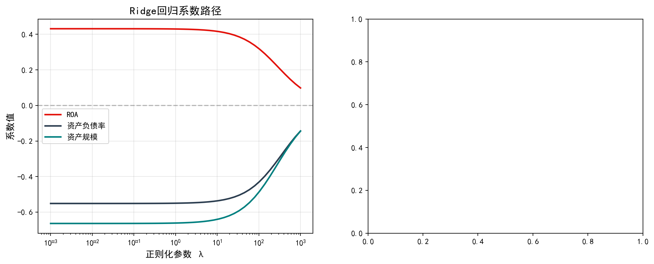

Ridge系数路径绘制完毕。下面在右侧面板绘制Lasso回归的系数路径，观察其特有的变量选择效应——某些系数会被精确压缩为零。

The Ridge coefficient path plot is complete. Next, we plot the Lasso regression coefficient paths in the right panel to observe its distinctive variable selection effect — some coefficients are shrunk exactly to zero.

# ----- 右图：Lasso系数路径 -----
# ----- Right panel: Lasso coefficient paths -----
lasso_path_axes = regularization_axes_array[1]                      # 选取右侧子图
# Select right subplot
for i, (name, color) in enumerate(zip(                              # 遍历每个变量
# Iterate over each variable
        regularization_variable_names_list,  # 变量名称列表
        # Variable name list
        regularization_plot_colors_list)):  # 对应颜色列表
        # Corresponding color list
    lasso_path_axes.plot(regularization_penalty_alphas_array,        # 绘制系数随λ变化曲线
    # Plot coefficient vs. λ curve
        lasso_coefficients_path_list[:, i],  # 第i个变量的Lasso系数路径
        # Lasso coefficient path for the i-th variable
        label=name, color=color, linewidth=2)  # 设置图例、颜色和线宽
        # Set legend, color, and line width
lasso_path_axes.set_xscale('log')                                   # x轴对数刻度
# Logarithmic scale for x-axis
lasso_path_axes.set_xlabel('正则化参数 λ', fontsize=12)               # x轴标签
# x-axis label
lasso_path_axes.set_ylabel('系数值', fontsize=12)                      # y轴标签
# y-axis label
lasso_path_axes.set_title('Lasso回归系数路径', fontsize=14)          # 标题
# Title
lasso_path_axes.legend()                                            # 图例
# Legend
lasso_path_axes.grid(True, alpha=0.3)                               # 网格线
# Grid lines
lasso_path_axes.axhline(y=0, color='gray', linestyle='--',         # 零值参考线
# Zero reference line
    alpha=0.5)  # 半透明显示
# Semi-transparent display

plt.tight_layout()                                                  # 自动调整布局
# Automatically adjust layout
plt.show()                                                          # 显示图表
# Display the figure

<Figure size 672x480 with 0 Axes>

图 11.2: 正则化路径: Ridge vs Lasso

从系数路径图可以清晰看到两种正则化方法的本质区别：

The coefficient path plots clearly reveal the essential difference between the two regularization methods:

print('关键观察:')                                                    # 输出观察结论
# Print observation conclusions
print('- Ridge: 系数逐渐收缩但不会变为零')                          # Ridge特点
# Ridge characteristic
print('- Lasso: 系数可以被压缩为精确的零(变量选择)')                  # Lasso特点
# Lasso characteristic

关键观察:
- Ridge: 系数逐渐收缩但不会变为零
- Lasso: 系数可以被压缩为精确的零(变量选择)

如表 11.6 所示,我们通过交叉验证选择最优正则化参数,并比较不同方法的性能。

As shown in 表 11.6, we select the optimal regularization parameter via cross-validation and compare the performance of different methods.

# ========== 导入所需库 ==========
# ========== Import required libraries ==========
from sklearn.linear_model import RidgeCV, LassoCV                   # 带交叉验证的正则化回归
# Regularized regression with cross-validation

# ========== 第1步：交叉验证选择最优λ ==========
# ========== Step 1: Select optimal λ via cross-validation ==========
cross_validated_ridge_model = RidgeCV(                              # 5折交叉验证选择Ridge最优λ
# 5-fold cross-validation to select optimal Ridge λ
    alphas=regularization_penalty_alphas_array, cv=5  # 候选λ值序列，5折交叉验证
    # Candidate λ values, 5-fold cross-validation
).fit(scaled_regularization_features_matrix,  # 拟合标准化特征数据
# Fit on standardized feature data
      regularization_target_array)  # 传入因变量完成拟合
# Pass in target to complete fitting
cross_validated_lasso_model = LassoCV(                              # 5折交叉验证选择Lasso最优λ
# 5-fold cross-validation to select optimal Lasso λ
    alphas=regularization_penalty_alphas_array, cv=5,  # 候选λ值序列，5折CV
    # Candidate λ values, 5-fold CV
    max_iter=10000  # 设置最大迭代次数确保收敛
    # Set max iterations to ensure convergence
).fit(scaled_regularization_features_matrix,  # 拟合标准化特征数据
# Fit on standardized feature data
      regularization_target_array)  # 传入因变量完成拟合
# Pass in target to complete fitting

Ridge/Lasso交叉验证拟合完毕。下面输出最优正则化参数与模型对比结果。

Ridge/Lasso cross-validation fitting is complete. Below we output the optimal regularization parameters and model comparison results.

表 11.6: 交叉验证选择最优正则化参数

# ========== 第2步：输出交叉验证结果 ==========
# ========== Step 2: Output cross-validation results ==========
print('=== 交叉验证结果 ===\n')                                      # 标题
# Title
print(f'Ridge最优λ: {cross_validated_ridge_model.alpha_:.4f}')     # Ridge最优惩罚参数
# Optimal Ridge penalty parameter
ridge_cv_r2_score = cross_validated_ridge_model.score(               # 计算Ridge交叉验证R²
# Compute Ridge cross-validated R²
    scaled_regularization_features_matrix,  # 传入特征矩阵
    # Pass in feature matrix
    regularization_target_array)  # 传入因变量计算R²
    # Pass in target to calculate R²
print(f'Ridge CV R²: {ridge_cv_r2_score:.4f}')  # 输出Ridge拟合优度
# Print Ridge goodness of fit
print(f'Ridge系数: {cross_validated_ridge_model.coef_.round(4)}')   # Ridge系数向量
# Ridge coefficient vector

print(f'\nLasso最优λ: {cross_validated_lasso_model.alpha_:.4f}')   # Lasso最优惩罚参数
# Optimal Lasso penalty parameter
lasso_cv_r2_score = cross_validated_lasso_model.score(               # 计算Lasso交叉验证R²
# Compute Lasso cross-validated R²
    scaled_regularization_features_matrix,  # 传入特征矩阵
    # Pass in feature matrix
    regularization_target_array)  # 传入因变量计算R²
    # Pass in target to calculate R²
print(f'Lasso CV R²: {lasso_cv_r2_score:.4f}')  # 输出Lasso拟合优度
# Print Lasso goodness of fit
print(f'Lasso系数: {cross_validated_lasso_model.coef_.round(4)}')   # Lasso系数向量
# Lasso coefficient vector

# ========== 第3步：与OLS基准模型对比 ==========
# ========== Step 3: Compare with OLS baseline model ==========
ordinary_least_squares_model = LinearRegression().fit(               # 拟合普通OLS模型
# Fit ordinary OLS model
    scaled_regularization_features_matrix,  # 传入标准化特征矩阵
    # Pass in standardized feature matrix
    regularization_target_array)  # 传入因变量完成OLS拟合
    # Pass in target to complete OLS fitting
ols_r2_score = ordinary_least_squares_model.score(                   # 计算OLS拟合优度
# Compute OLS goodness of fit
    scaled_regularization_features_matrix,  # 传入特征矩阵
    # Pass in feature matrix
    regularization_target_array)  # 传入因变量计算R²
    # Pass in target to calculate R²
print(f'\nOLS R²: {ols_r2_score:.4f}')  # 输出OLS拟合优度
# Print OLS goodness of fit
print(f'OLS系数: {ordinary_least_squares_model.coef_.round(4)}')     # OLS系数向量
# OLS coefficient vector

=== 交叉验证结果 ===

Ridge最优λ: 104.8113
Ridge CV R²: 0.0955
Ridge系数: [ 0.3158 -0.4271 -0.4817]

Lasso最优λ: 0.3728
Lasso CV R²: 0.0580
Lasso系数: [ 0.0476 -0.2565 -0.2419]

OLS R²: 0.1022
OLS系数: [ 0.4314 -0.5515 -0.6639]

表 11.6 的交叉验证结果清晰地展示了三种方法的差异。Ridge回归通过5折交叉验证选择的最优惩罚参数\(\lambda\)为104.8113，对应的R²为0.0955，系数为[0.3158, -0.4271, -0.4817]——可以看到三个系数都被显著压缩但均不为零。Lasso回归的最优\(\lambda\)为0.3728，R²为0.0580，系数为[0.0476, -0.2565, -0.2419]——第一个系数（log_assets）已被压缩至接近零（0.0476），体现了Lasso的变量选择特性。作为基准对比，OLS回归的R²为0.1022，系数为[0.4314, -0.5515, -0.6639]——虽然拟合优度最高，但系数绝对值也最大。这组对比揭示了正则化的核心思想：OLS追求训练集上的最佳拟合，但可能过度拟合导致泛化能力差；正则化以牺牲少量训练集拟合优度（R²从0.1022分别下降到0.0955和0.0580）为代价，换取更稳定、更可靠的系数估计，这在高维数据或存在多重共线性的场景中尤为重要。

The cross-validation results in 表 11.6 clearly demonstrate the differences among the three methods. Ridge regression, with its optimal penalty parameter \(\lambda\) of 104.8113 selected by 5-fold cross-validation, yields an R² of 0.0955 and coefficients of [0.3158, -0.4271, -0.4817] — all three coefficients are substantially shrunk but none are zero. Lasso regression has an optimal \(\lambda\) of 0.3728, an R² of 0.0580, and coefficients of [0.0476, -0.2565, -0.2419] — the first coefficient (log_assets) has been shrunk to near zero (0.0476), reflecting Lasso’s variable selection property. As a baseline comparison, OLS regression achieves the highest R² of 0.1022, with coefficients of [0.4314, -0.5515, -0.6639] — although the goodness of fit is highest, the absolute values of the coefficients are also the largest. This comparison reveals the core idea of regularization: OLS seeks the best fit on the training set but may overfit, leading to poor generalization; regularization sacrifices a small amount of training-set goodness of fit (R² drops from 0.1022 to 0.0955 and 0.0580, respectively) in exchange for more stable and reliable coefficient estimates, which is especially important in high-dimensional data or scenarios with multicollinearity. ## 启发式思考题 (Heuristic Problems) {#sec-heuristic-problems-ch11}

1. 线性概率模型的陷阱 (The Linear Probability Model Trap) - 操作：找一个二分类数据集（\(Y \in \{0,1\}\)），强行用普通线性回归 (OLS) 拟合它 (\(Y = \beta X + \epsilon\))。 - 预测：用模型预测几个极端样本的概率。 - 结果：你会发现预测值可能出现 \(P > 1\)（如 1.2）或 \(P < 0\)（如 -0.3）。这在概率世界是荒谬的。 - 反思：这就是为什么你需要 S 型的 Logistic 函数，把直线弯曲成曲线，限制在 \([0,1]\) 区间内。

1. The Linear Probability Model Trap - Task: Find a binary classification dataset (\(Y \in \{0,1\}\)) and force-fit it with ordinary linear regression (OLS) (\(Y = \beta X + \epsilon\)). - Prediction: Use the model to predict probabilities for several extreme observations. - Result: You will find that predicted values may exceed \(P > 1\) (e.g., 1.2) or fall below \(P < 0\) (e.g., -0.3). This is absurd in the world of probabilities. - Reflection: This is precisely why you need the S-shaped Logistic function — it bends the straight line into a curve, confining outputs to the \([0,1]\) interval.

图 11.3 直观展示了线性概率模型的致命缺陷。

图 11.3 visually demonstrates the fatal flaw of the linear probability model.

# ========== 导入所需库 ==========
# ========== Import required libraries ==========
import numpy as np                                                  # 数值计算
# NumPy for numerical computation
import matplotlib.pyplot as plt                                     # 绘图
# Matplotlib for plotting
from sklearn.linear_model import LinearRegression, LogisticRegression  # 线性+逻辑回归
# Import linear and logistic regression from scikit-learn
import platform                                                     # 平台检测
# Platform detection module

# ========== 中文字体设置 ==========
# ========== Chinese font configuration ==========
if platform.system() == 'Linux':                                    # Linux字体配置
# Linux font configuration
    plt.rcParams['font.sans-serif'] = ['Source Han Serif SC', 'SimHei']  # 设置Linux中文字体
    # Set Chinese fonts for Linux
else:                                                               # Windows字体配置
# Windows font configuration
    plt.rcParams['font.sans-serif'] = ['SimHei', 'Microsoft YaHei']  # 设置Windows中文字体
    # Set Chinese fonts for Windows
plt.rcParams['axes.unicode_minus'] = False                          # 正常显示负号
# Enable proper display of minus signs

# ========== 第1步：生成模拟违约数据 ==========
# ========== Step 1: Generate simulated default data ==========
# 注：此处使用模拟数据是为演示LPM的理论缺陷，属于统计性质展示
# Note: Simulated data is used here to demonstrate the theoretical flaws of LPM; this is a statistical property demonstration
np.random.seed(42)                                                  # 设置随机种子
# Set random seed for reproducibility
sample_size = 200                                                   # 样本量200家企业
# Sample size: 200 firms
financial_health_score = np.random.uniform(-3, 3, sample_size)      # 财务健康指数（均匀分布）
# Financial health score (uniform distribution)
true_default_probability = 1 / (1 + np.exp(                         # 真实违约概率（Logistic函数）
    -(-1.5 + 1.2 * financial_health_score)))  # Logistic函数的线性部分参数
# True default probability via the Logistic function; parameters of the linear component
observed_default_indicator = np.random.binomial(                    # 生成0/1违约二分类结果
    1, true_default_probability)  # 单次伯努利试验，以真实概率生成
# Generate binary default indicator via a single Bernoulli trial using true probability

模拟违约数据生成完毕。下面分别用线性概率模型和Logistic回归进行拟合，并在扩展范围内预测概率。

The simulated default data has been generated. Next, we fit both the linear probability model and logistic regression, and predict probabilities over an extended range.

# ========== 第2步：分别拟合LPM和Logistic模型 ==========
# ========== Step 2: Fit LPM and Logistic models separately ==========
linear_probability_model = LinearRegression()                       # 创建OLS线性回归（LPM）
# Create an OLS linear regression model (LPM)
linear_probability_model.fit(                                       # 拟合LPM
    financial_health_score.reshape(-1, 1),  # 特征转为列向量
    observed_default_indicator)  # 传入标签完成拟合
# Fit the LPM: reshape features to column vector and pass labels

logistic_regression_model = LogisticRegression()                    # 创建Logistic回归
# Create a Logistic regression model
logistic_regression_model.fit(                                      # 拟合Logistic
    financial_health_score.reshape(-1, 1),  # 特征转为列向量
    observed_default_indicator)  # 传入标签完成拟合
# Fit the Logistic model: reshape features to column vector and pass labels

# ========== 第3步：在扩展范围内预测 ==========
# ========== Step 3: Predict over an extended range ==========
prediction_range_array = np.linspace(-5, 5, 300).reshape(-1, 1)     # 预测区间[-5,5]包含极端值
# Prediction range [-5, 5] including extreme values
lpm_predicted_probability = linear_probability_model.predict(       # LPM预测（可能超出[0,1]）
    prediction_range_array)  # 传入预测范围数组
# LPM prediction (may exceed [0,1]); pass the prediction range array
logistic_predicted_probability = (logistic_regression_model         # Logistic预测（始终在[0,1]）
    .predict_proba(prediction_range_array)[:, 1])  # 取正类概率列
# Logistic prediction (always within [0,1]); extract the positive-class probability column

模拟数据生成及两种模型的预测已完成。下面绘制对比图，直观展示线性概率模型产生超出[0,1]范围的”荒谬概率”的缺陷，而Logistic回归始终保持在合理区间内。

Simulated data generation and predictions from both models are complete. Next, we create a comparison plot to visually demonstrate the flaw of the linear probability model producing “absurd probabilities” outside the [0,1] range, while logistic regression always stays within a reasonable interval.

# ========== 第4步：创建画布并绘制LPM与Logistic预测曲线 ==========
# ========== Step 4: Create canvas and plot LPM vs. Logistic prediction curves ==========
comparison_figure, comparison_axes = plt.subplots(1, 1, figsize=(10, 6))  # 创建画布
# Create a figure with a single subplot

# 散点图：观测的违约/非违约数据
# Scatter plot: observed default/non-default data
comparison_axes.scatter(  # 绘制观测数据散点
    financial_health_score, observed_default_indicator,  # X为健康指数，Y为违约标记
    alpha=0.3, color='gray', s=20, label='观测数据'                  # 灰色半透明散点
)
# Plot observed data points: X = health score, Y = default indicator; gray semi-transparent dots

# LPM预测线（红色虚线）
# LPM prediction line (red dashed)
comparison_axes.plot(  # 绘制LPM预测概率曲线
    prediction_range_array, lpm_predicted_probability,  # X为特征范围，Y为LPM预测值
    color='#E3120B', linewidth=2.5, linestyle='--',                  # 红色虚线
    label='线性概率模型 (OLS)'  # 设置LPM图例标签
)
# Plot LPM predicted probability curve: X = feature range, Y = LPM predicted values; red dashed line

# Logistic预测线（青色实线）
# Logistic prediction line (teal solid)
comparison_axes.plot(  # 绘制Logistic预测概率曲线
    prediction_range_array, logistic_predicted_probability,  # X为特征范围，Y为Logistic预测值
    color='#008080', linewidth=2.5, label='Logistic回归'             # 青色实线
)
# Plot Logistic predicted probability curve: X = feature range, Y = Logistic predicted values; teal solid line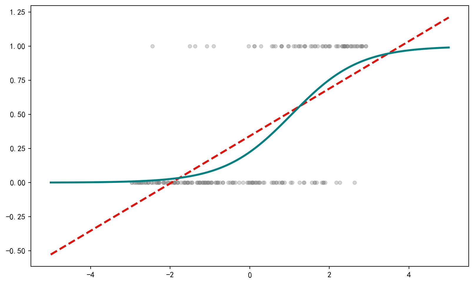

散点图和两种模型的拟合曲线已绘制。下面标注LPM的概率越界区域（预测概率超出\([0,1]\)范围的”荒谬区域”），直观展示线性概率模型的理论缺陷。

The scatter plot and fitted curves from both models have been drawn. Next, we annotate the LPM’s out-of-bound probability regions (where predicted probabilities exceed the \([0,1]\) range — the “absurd zones”) to visually highlight the theoretical deficiency of the linear probability model.

# ========== 标注概率越界区域并完成图表 ==========
# ========== Annotate out-of-bound probability regions and finalize the chart ==========
comparison_axes.axhline(y=0, color='black', linewidth=0.8,          # y=0参考线
    linestyle='-')  # 实线样式
# Draw reference line at y=0; solid line style
comparison_axes.axhline(y=1, color='black', linewidth=0.8,          # y=1参考线
    linestyle='-')  # 实线样式
# Draw reference line at y=1; solid line style
comparison_axes.fill_between(                                        # 填充P>1的荒谬区域
    prediction_range_array.flatten(), 1,  # X坐标展平，上界为1
    lpm_predicted_probability.flatten(),  # 下界为LPM预测值
    where=lpm_predicted_probability.flatten() > 1,  # 仅填充预测超过1的区域
    alpha=0.3, color='#E3120B', label='P > 1 (荒谬区域)'  # 红色半透明填充，标注图例
)
# Fill the absurd region where P > 1: flatten X coords, upper bound = 1, lower bound = LPM prediction
comparison_axes.fill_between(                                        # 填充P<0的荒谬区域
    prediction_range_array.flatten(), 0,  # X坐标展平，下界为0
    lpm_predicted_probability.flatten(),  # 上界为LPM预测值
    where=lpm_predicted_probability.flatten() < 0,  # 仅填充预测低于0的区域
    alpha=0.3, color='#E3120B'  # 红色半透明填充
)
# Fill the absurd region where P < 0: flatten X coords, lower bound = 0, upper bound = LPM prediction

comparison_axes.set_xlabel('财务健康指数', fontsize=12)               # x轴标签
# Set x-axis label: Financial Health Score
comparison_axes.set_ylabel('违约概率', fontsize=12)                   # y轴标签
# Set y-axis label: Default Probability
comparison_axes.set_title('线性概率模型 vs Logistic回归', fontsize=14)  # 标题
# Set title: Linear Probability Model vs Logistic Regression
comparison_axes.legend(loc='upper left', fontsize=10)                # 图例
# Display legend at upper left
comparison_axes.set_ylim(-0.5, 1.5)                                  # y轴范围（展示越界效果）
# Set y-axis range to show the out-of-bound effect
comparison_axes.grid(True, alpha=0.3)                                # 网格线
# Add grid lines
plt.tight_layout()                                                   # 自动调整
# Auto-adjust layout
plt.show()                                                           # 显示图表
# Display the chart

<Figure size 672x480 with 0 Axes>

图 11.3: 线性概率模型的陷阱：预测概率超出[0,1]范围

LPM与Logistic回归的对比图绘制完成。下面统计线性概率模型中预测概率越界的比例。

The comparison chart of LPM versus logistic regression is complete. Next, we compute the proportion of out-of-bound predicted probabilities from the linear probability model.

# ========== 第5步：统计LPM越界预测比例 ==========
# ========== Step 5: Compute the proportion of LPM out-of-bound predictions ==========
out_of_range_count = np.sum(                                         # 统计越界预测点数
    (lpm_predicted_probability < 0) | (lpm_predicted_probability > 1)  # 预测概率小于0或大于1的布尔条件
)
# Count the number of out-of-range prediction points: predicted probability < 0 or > 1
print(f'线性概率模型在{len(prediction_range_array)}个预测点中,')     # 输出总预测点数
# Print total number of prediction points
print(f'有{out_of_range_count}个点的预测概率超出[0,1]范围')           # 输出越界数量
# Print number of points with predicted probability outside [0,1]
print(f'({out_of_range_count/len(prediction_range_array)*100:.1f}%)')  # 越界百分比
# Print percentage of out-of-range predictions
print('这正是Logistic回归存在的核心意义。')  # 输出核心结论
# Print core conclusion: this is the fundamental reason logistic regression exists

线性概率模型在300个预测点中,
有128个点的预测概率超出[0,1]范围
(42.7%)
这正是Logistic回归存在的核心意义。

运行结果令人震惊：在300个预测点中，线性概率模型有128个点（占42.7%）的预测概率超出了\([0,1]\)的合法范围——这意味着近一半的预测结果在概率意义上是荒谬的。当财务健康指数取极端值时，LPM会给出诸如\(P=-0.3\)或\(P=1.2\)这样”负概率”和”超百分之百概率”的结果。相比之下，Logistic回归通过Sigmoid函数\(\sigma(z) = \frac{1}{1+e^{-z}}\)将输出自动约束在\((0,1)\)区间内，无论输入多么极端，预测概率始终是合理的。这正是为什么在二分类问题中，Logistic回归是线性概率模型的必要升级。

The results are striking: out of 300 prediction points, the linear probability model produces 128 points (42.7%) with predicted probabilities outside the legitimate \([0,1]\) range — meaning nearly half of all predictions are probabilistically absurd. When the financial health score takes extreme values, the LPM yields results such as \(P=-0.3\) or \(P=1.2\), i.e., “negative probabilities” and “probabilities exceeding 100%.” In contrast, logistic regression uses the Sigmoid function \(\sigma(z) = \frac{1}{1+e^{-z}}\) to automatically constrain outputs within the \((0,1)\) interval; no matter how extreme the input, the predicted probability always remains sensible. This is precisely why, for binary classification problems, logistic regression is the necessary upgrade over the linear probability model.

2. 完美分离的毁灭性 (Perfect Separation) - 实验：生成一个数据集，其中 \(X > 5\) 时 \(Y\) 总是 1，\(X \le 5\) 时 \(Y\) 总是 0。 - 观察：运行 Logistic 回归。你会发现 \(X\) 的系数巨大无比（比如 5000），标准误也是天文数字，p 值接近 1（不显著）。 - 原因：模型为了让似然函数最大化，试图把 logistic 曲线变垂直（斜率无穷大）。 - 启示：当模型完全准确时，传统的统计推断反而会崩溃。这时需要正则化（Penalization）。

2. The Destructiveness of Perfect Separation - Experiment: Generate a dataset where \(Y\) is always 1 when \(X > 5\) and always 0 when \(X \le 5\). - Observation: Run logistic regression. You will find that the coefficient for \(X\) is astronomically large (e.g., 5000), the standard error is also astronomical, and the p-value is close to 1 (not significant). - Reason: In order to maximize the likelihood function, the model attempts to make the logistic curve vertical (infinite slope). - Implication: When the model achieves perfect accuracy, traditional statistical inference actually breaks down. This is when regularization (penalization) is needed.

图 11.4 展示了完美分离对Logistic回归的毁灭性影响。

图 11.4 illustrates the devastating impact of perfect separation on logistic regression.

# ========== 导入所需库 ==========
# ========== Import required libraries ==========
import numpy as np                    # 数值计算库
# NumPy for numerical computation
import statsmodels.api as sm          # 统计建模库（Logit模型）
# Statsmodels for statistical modeling (Logit model)
import matplotlib.pyplot as plt       # 数据可视化库
# Matplotlib for data visualization
import warnings                       # 警告管理模块
# Warnings management module
warnings.filterwarnings('ignore')     # 忽略收敛警告，保持输出整洁
# Suppress convergence warnings to keep output clean

# ========== 第1步：构造完美分离数据集 ==========
# ========== Step 1: Construct a perfectly separated dataset ==========
# 完美分离：当特征X能完美区分Y=0和Y=1时，MLE不收敛
# Perfect separation: when feature X can perfectly distinguish Y=0 from Y=1, MLE does not converge
np.random.seed(42)                    # 设置随机种子，确保结果可重复
# Set random seed for reproducibility
# --- 组1：X <= 5 的样本全部标记为 Y=0（正常企业）---
# --- Group 1: All samples with X <= 5 are labeled Y=0 (normal firms) ---
group_zero_feature_array = np.random.uniform(0, 5, 50)    # 生成50个[0,5]均匀分布特征值
# Generate 50 feature values uniformly distributed over [0, 5]
group_zero_label_array = np.zeros(50)                      # 对应标签全为0
# Corresponding labels are all 0
# --- 组2：X > 5 的样本全部标记为 Y=1（违约企业）---
# --- Group 2: All samples with X > 5 are labeled Y=1 (defaulted firms) ---
group_one_feature_array = np.random.uniform(5.01, 10, 50)  # 生成50个(5,10]均匀分布特征值
# Generate 50 feature values uniformly distributed over (5, 10]
group_one_label_array = np.ones(50)                        # 对应标签全为1
# Corresponding labels are all 1

# ========== 第2步：合并两组数据 ==========
# ========== Step 2: Merge the two groups ==========
perfect_separation_feature_array = np.concatenate(         # 拼接特征数组
    [group_zero_feature_array, group_one_feature_array]    # 合并两组特征值
)
# Concatenate feature arrays from both groups
perfect_separation_label_array = np.concatenate(           # 拼接标签数组
    [group_zero_label_array, group_one_label_array]        # 合并两组标签
)
# Concatenate label arrays from both groups

完美分离数据集构造完毕。下面尝试对该数据拟合Logistic回归，观察MLE不收敛现象。

The perfectly separated dataset is now constructed. Next, we attempt to fit logistic regression to this data and observe the MLE non-convergence phenomenon.

# ========== 第3步：尝试对完美分离数据拟合Logistic回归 ==========
# ========== Step 3: Attempt to fit logistic regression on perfectly separated data ==========
design_matrix_with_constant = sm.add_constant(perfect_separation_feature_array)  # 添加截距列
# Add an intercept column to the design matrix
try:  # 尝试拟合完美分离数据（可能不收敛）
# Try fitting on perfectly separated data (may not converge)
    perfect_separation_logistic_model = sm.Logit(          # 构建Logit模型
        perfect_separation_label_array, design_matrix_with_constant  # 传入因变量和设计矩阵
    ).fit(maxiter=100, disp=0)                             # 拟合模型，最多迭代100次，关闭输出
    # Build and fit the Logit model: pass dependent variable and design matrix; max 100 iterations, suppress output

    print('=== 完美分离下的Logistic回归结果 ===')          # 打印标题
    # Print header: Logistic regression results under perfect separation
    print(f'X的系数: {perfect_separation_logistic_model.params[1]:.2f} (极大!)')    # 系数趋于无穷
    # Print coefficient of X (tends to infinity)
    print(f'X的标准误: {perfect_separation_logistic_model.bse[1]:.2f} (极大!)')     # 标准误趋于无穷
    # Print standard error of X (tends to infinity)
    print(f'X的p值: {perfect_separation_logistic_model.pvalues[1]:.4f} (不显著)')   # p值失去意义
    # Print p-value of X (loses significance)
    print('\n结论: 完美分离导致MLE不收敛,系数和标准误趋向无穷大')  # 打印结论
    # Print conclusion: perfect separation causes MLE non-convergence; coefficients and standard errors tend to infinity
except Exception as estimation_error:                      # 捕获拟合失败异常
# Catch fitting failure exception
    print(f'拟合失败: {estimation_error}')                 # 打印错误信息
    # Print the error message
    print('完美分离导致极大似然估计不存在有限解')           # 解释原因
    # Explain: perfect separation causes MLE to have no finite solution

=== 完美分离下的Logistic回归结果 ===
X的系数: 181.66 (极大!)
X的标准误: 38115.78 (极大!)
X的p值: 0.9962 (不显著)

结论: 完美分离导致MLE不收敛,系数和标准误趋向无穷大

上面的数值结果表明，完美分离导致系数和标准误趋于无穷大，统计推断完全失效。下面通过可视化对比完美分离数据与正常数据的Logistic拟合曲线，直观展示这一问题的严重性及其解决思路。首先预计算绘图所需的预测数据和正常对照组模型：

The numerical results above demonstrate that perfect separation causes coefficients and standard errors to tend toward infinity, rendering statistical inference completely invalid. Below, we visually compare the logistic fitted curves for perfectly separated data versus normal data, intuitively illustrating the severity of this problem and the approach to resolving it. First, we precompute the prediction data and the normal control group model needed for plotting:

# ========== 第4步：预计算可视化所需数据 ==========
# ========== Step 4: Precompute data needed for visualization ==========
plot_x_range = np.linspace(-1, 11, 300)                    # 生成预测用X值范围
# Generate X value range for prediction
plot_design_matrix = sm.add_constant(plot_x_range)         # 添加截距列
# Add intercept column
has_perfect_separation_prediction = False                  # 初始化预测成功标志
# Initialize prediction success flag
try:                                                       # 尝试用完美分离模型预测
# Try prediction with the perfectly separated model
    predicted_probability_curve = perfect_separation_logistic_model.predict(plot_design_matrix)  # 计算预测概率
    # Compute predicted probabilities
    has_perfect_separation_prediction = True                # 标记预测成功
    # Mark prediction as successful
except Exception:                                          # 若模型未成功拟合则跳过
# If the model was not successfully fitted, skip
    pass                                                   # 预测失败则保持标志为False
    # Keep flag as False if prediction fails

# ========== 第5步：生成正常数据对照组 ==========
# ========== Step 5: Generate normal data control group ==========
np.random.seed(123)                                        # 设置随机种子
# Set random seed
normal_feature_array = np.random.uniform(0, 10, 100)       # 生成100个[0,10]均匀分布特征值
# Generate 100 feature values uniformly distributed over [0, 10]
normal_probability_array = 1 / (1 + np.exp(-(normal_feature_array - 5)))  # 用Sigmoid函数计算真实概率
# Compute true probabilities using the Sigmoid function
normal_label_array = np.random.binomial(1, normal_probability_array)      # 按概率生成0/1标签（有重叠）
# Generate 0/1 labels according to probabilities (with class overlap)
normal_design_matrix = sm.add_constant(normal_feature_array)  # 添加截距列
# Add intercept column
normal_logistic_model = sm.Logit(normal_label_array, normal_design_matrix).fit(disp=0)  # 拟合正常数据Logit模型
# Fit Logit model on normal data
normal_predicted_array = normal_logistic_model.predict(sm.add_constant(plot_x_range))  # 正常模型预测概率
# Predicted probabilities from the normal model

预计算完成。下面以双面板对比图展示完美分离与正常数据在Logistic回归拟合上的差异：

Precomputation is complete. Below, we present a two-panel comparison chart showing the differences in logistic regression fitting between perfectly separated data and normal data:

# ========== 第6步：创建画布并绘制左侧面板（完美分离） ==========
# ========== Step 6: Create canvas and plot the left panel (perfect separation) ==========
separation_figure, separation_axes_array = plt.subplots(1, 2, figsize=(14, 5))  # 创建1行2列子图
# Create a figure with 1 row and 2 columns of subplots

# --- 左图：完美分离数据和拟合曲线 ---
# --- Left panel: Perfectly separated data and fitted curve ---
data_axes = separation_axes_array[0]                       # 获取左侧子图
# Get the left subplot
data_axes.scatter(                                         # 绘制Y=0组散点
    group_zero_feature_array, group_zero_label_array,      # X和Y坐标
    color='#2C3E50', alpha=0.6, s=40, label='Y=0 (正常)'  # 深蓝色，标签为正常
)
# Plot scatter points for the Y=0 group: dark blue, labeled as normal
data_axes.scatter(                                         # 绘制Y=1组散点
    group_one_feature_array, group_one_label_array,        # X和Y坐标
    color='#E3120B', alpha=0.6, s=40, label='Y=1 (违约)'  # 红色，标签为违约
)
# Plot scatter points for the Y=1 group: red, labeled as default
if has_perfect_separation_prediction:                      # 若完美分离模型预测成功
# If the perfectly separated model prediction succeeded
    data_axes.plot(                                        # 绘制拟合曲线
        plot_x_range, predicted_probability_curve,         # X轴为特征值，Y轴为预测概率
        'g-', linewidth=2, label='Logistic拟合(近似阶跃)'  # 绿色实线
    )
    # Plot the fitted curve: green solid line, labeled as Logistic fit (near step function)
data_axes.axvline(x=5, color='gray', linestyle='--', alpha=0.5, label='分离边界 X=5')  # 绘制分离边界线
# Draw the separation boundary line at X=5
data_axes.set_xlabel('X (特征变量)', fontsize=12)          # 设置X轴标签
# Set x-axis label: X (feature variable)
data_axes.set_ylabel('Y (0/1)', fontsize=12)               # 设置Y轴标签
# Set y-axis label: Y (0/1)
data_axes.set_title('完美分离：数据被X=5完美分开', fontsize=13)  # 设置子图标题
# Set subplot title: Perfect separation — data perfectly divided at X=5
data_axes.legend(fontsize=9)                               # 显示图例
# Display legend
data_axes.grid(True, alpha=0.3)                            # 添加网格线
# Add grid lines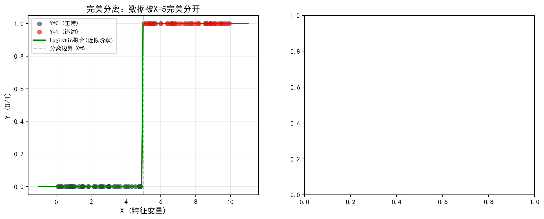

完美分离数据的可视化完成。接下来在右侧面板绘制正常数据（类别之间存在重叠）时Logistic回归的拟合结果，作为对照展示正常情况下系数的合理估计。

Visualization of the perfectly separated data is complete. Next, we plot the logistic regression fit on normal data (where classes overlap) in the right panel, serving as a control to show reasonable coefficient estimates under normal conditions.

# --- 右图：正常数据的Logistic回归（有重叠区域）---
# --- Right panel: Logistic regression on normal data (with overlapping regions) ---
normal_axes = separation_axes_array[1]                     # 获取右侧子图
# Get the right subplot
normal_axes.scatter(                                       # 绘制Y=0的散点
    normal_feature_array[normal_label_array == 0],         # 筛选标签为0的样本
    normal_label_array[normal_label_array == 0],           # 对应的Y值
    color='#2C3E50', alpha=0.6, s=40, label='Y=0'         # 深蓝色散点
)
# Plot scatter points for Y=0: filter samples with label 0; dark blue dots
normal_axes.scatter(                                       # 绘制Y=1的散点
    normal_feature_array[normal_label_array == 1],         # 筛选标签为1的样本
    normal_label_array[normal_label_array == 1],           # 对应的Y值
    color='#E3120B', alpha=0.6, s=40, label='Y=1'         # 红色散点
)
# Plot scatter points for Y=1: filter samples with label 1; red dots
normal_axes.plot(                                          # 绘制S形拟合曲线
    plot_x_range, normal_predicted_array,                  # X轴为特征值，Y轴为预测概率
    '#008080', linewidth=2, label='Logistic拟合(正常S曲线)'  # 青色实线
)
# Plot the S-shaped fitted curve: X = feature values, Y = predicted probabilities; teal solid line
normal_axes.set_xlabel('X (特征变量)', fontsize=12)        # 设置X轴标签
# Set x-axis label: X (feature variable)
normal_axes.set_ylabel('P(Y=1)', fontsize=12)              # 设置Y轴标签（概率）
# Set y-axis label: P(Y=1)
normal_axes.set_title(                                     # 设置子图标题，展示正常估计结果
    f'正常数据: \u03b2={normal_logistic_model.params[1]:.2f}, '     # β系数（有限值）
    f'SE={normal_logistic_model.bse[1]:.2f}', fontsize=13           # 标准误（有限值）
)
# Set subplot title showing normal estimation results: β coefficient (finite) and SE (finite)
normal_axes.legend(fontsize=9)                             # 显示图例
# Display legend
normal_axes.grid(True, alpha=0.3)                          # 添加网格线
# Add grid lines

plt.tight_layout()                                         # 自动调整子图间距
# Auto-adjust subplot spacing
plt.show()                                                 # 显示图形
# Display the figure

<Figure size 672x480 with 0 Axes>

图 11.4: 完美分离导致Logistic回归系数爆炸

可视化对比已完成。下面输出定量对比结论。

The visual comparison is complete. Below, we output the quantitative comparison conclusion.

print(f'\n正常数据: \u03b2={normal_logistic_model.params[1]:.2f}, '     # 打印正常数据的β系数
      f'SE={normal_logistic_model.bse[1]:.2f}, '                        # 打印正常数据的标准误
      f'p={normal_logistic_model.pvalues[1]:.4f}')                      # 打印正常数据的p值
# Print normal data results: β coefficient, standard error, and p-value
print('对比可见: 完美分离时系数爆炸, 传统统计推断失效')     # 对比结论
# Comparison conclusion: under perfect separation, coefficients explode and traditional statistical inference fails
print('解决方案: 使用Firth惩罚回归或正则化方法')            # 建议解决方案
# Recommended solution: use Firth penalized regression or regularization methods


正常数据: β=1.11, SE=0.21, p=0.0000
对比可见: 完美分离时系数爆炸, 传统统计推断失效
解决方案: 使用Firth惩罚回归或正则化方法

11.6 习题 (Exercises)

习题1: Logistic回归的似然函数

Exercise 1: The Likelihood Function of Logistic Regression

推导Logistic回归的对数似然函数
Derive the log-likelihood function of logistic regression.
对参数\(\beta_j\)求一阶导数(得分函数)
Take the first derivative with respect to the parameter \(\beta_j\) (the score function).
解释为什么需要数值方法求解
Explain why numerical methods are needed to solve it.

习题2: 财务困境预测

Exercise 2: Financial Distress Prediction

使用本地上市公司数据:

Using local listed company data:

选择适当的财务指标作为预测变量
建立Logistic回归模型预测ST风险
计算并解释几率比
评估模型性能(AUC、混淆矩阵)
Select appropriate financial indicators as predictor variables.
Build a logistic regression model to predict ST (special treatment) risk.
Calculate and interpret odds ratios.
Evaluate model performance (AUC, confusion matrix).

习题3: Poisson回归与过度离散

Exercise 3: Poisson Regression and Overdispersion

解释Poisson分布的方差等于均值假设
如何检验过度离散?
比较Poisson回归和负二项回归的结果
Explain the Poisson distribution’s assumption that the variance equals the mean.
How do you test for overdispersion?
Compare the results of Poisson regression and negative binomial regression.

习题4: 正则化方法比较

Exercise 4: Comparison of Regularization Methods

解释Ridge和Lasso惩罚项的几何含义
为什么Lasso可以产生稀疏解?
使用交叉验证选择最优λ
比较不同方法的预测性能
Explain the geometric interpretation of Ridge and Lasso penalty terms.
Why can Lasso produce sparse solutions?
Use cross-validation to select the optimal λ.
Compare the predictive performance of different methods. ## 解答 (Solutions) {#sec-solutions-ch11}

习题1解答

Solution to Exercise 1

(a) 对数似然函数推导

(a) Derivation of the Log-Likelihood Function

设 \(Y_i \in \{0,1\}\)，\(P(Y_i=1) = p_i\)。由于 \(Y_i\) 服从伯努利分布，单个观测的概率质量函数为:

Let \(Y_i \in \{0,1\}\) and \(P(Y_i=1) = p_i\). Since \(Y_i\) follows a Bernoulli distribution, the probability mass function for a single observation is:

\[P(Y_i = y_i) = p_i^{y_i}(1-p_i)^{1-y_i}\]

对于 \(n\) 个独立观测，似然函数为:

For \(n\) independent observations, the likelihood function is:

\[L(\boldsymbol{\beta}) = \prod_{i=1}^n p_i^{y_i}(1-p_i)^{1-y_i}\]

取对数:

Taking the logarithm:

\[\ell(\boldsymbol{\beta}) = \sum_{i=1}^n \left[y_i \ln p_i + (1-y_i)\ln(1-p_i)\right]\]

代入 \(p_i = \frac{e^{\eta_i}}{1+e^{\eta_i}}\)（其中 \(\eta_i = \mathbf{x}_i'\boldsymbol{\beta}\)），注意到:

Substituting \(p_i = \frac{e^{\eta_i}}{1+e^{\eta_i}}\) (where \(\eta_i = \mathbf{x}_i'\boldsymbol{\beta}\)), we note that:

\(\ln p_i = \ln \frac{e^{\eta_i}}{1+e^{\eta_i}} = \eta_i - \ln(1+e^{\eta_i})\)
\(\ln(1-p_i) = \ln \frac{1}{1+e^{\eta_i}} = -\ln(1+e^{\eta_i})\)

代入得:

Substituting yields:

\[\ell(\boldsymbol{\beta}) = \sum_{i=1}^n \left[y_i \eta_i - \ln(1+e^{\eta_i})\right]\]

(b) 得分函数(一阶导数)

(b) The Score Function (First Derivative)

对 \(\beta_j\) 求偏导:

Taking the partial derivative with respect to \(\beta_j\):

\[\frac{\partial \ell}{\partial \beta_j} = \sum_{i=1}^n \left[y_i x_{ij} - \frac{e^{\eta_i}}{1+e^{\eta_i}} x_{ij}\right] = \sum_{i=1}^n (y_i - p_i) x_{ij}\]

矩阵形式: \(\frac{\partial \ell}{\partial \boldsymbol{\beta}} = \mathbf{X}'(\mathbf{y} - \mathbf{p})\)

In matrix form: \(\frac{\partial \ell}{\partial \boldsymbol{\beta}} = \mathbf{X}'(\mathbf{y} - \mathbf{p})\)

(c) 需要数值方法的原因

(c) Why Numerical Methods Are Required

得分方程 \(\mathbf{X}'(\mathbf{y} - \mathbf{p}) = \mathbf{0}\) 是非线性的，因为 \(p_i = \frac{e^{\mathbf{x}_i'\boldsymbol{\beta}}}{1+e^{\mathbf{x}_i'\boldsymbol{\beta}}}\) 是 \(\boldsymbol{\beta}\) 的非线性函数。不存在闭式解，需要使用Newton-Raphson或Fisher Scoring迭代算法求解。

The score equation \(\mathbf{X}'(\mathbf{y} - \mathbf{p}) = \mathbf{0}\) is nonlinear because \(p_i = \frac{e^{\mathbf{x}_i'\boldsymbol{\beta}}}{1+e^{\mathbf{x}_i'\boldsymbol{\beta}}}\) is a nonlinear function of \(\boldsymbol{\beta}\). No closed-form solution exists, and iterative algorithms such as Newton-Raphson or Fisher Scoring must be used.

数值验证: 使用本地数据验证似然函数的计算。

Numerical Verification: Verify the computation of the likelihood function using local data.

# ========== 导入所需库 ==========
# ========== Import required libraries ==========
import numpy as np                    # 数值计算库
                                      # Numerical computation library
import statsmodels.api as sm          # 统计建模库
                                      # Statistical modeling library
import platform                       # 平台检测模块
                                      # Platform detection module

# ========== 第1步：读取本地财务数据 ==========
# ========== Step 1: Read local financial data ==========
if platform.system() == 'Windows':                         # 判断操作系统
                                                           # Detect operating system
    data_path = 'C:/qiufei/data/stock'                     # Windows数据路径
                                                           # Windows data path
else:  # 非Windows系统(Linux)
       # Non-Windows system (Linux)
    data_path = '/home/ubuntu/r2_data_mount/qiufei/data/stock'  # Linux数据路径
                                                                 # Linux data path

import pandas as pd                                        # 数据处理库
                                                           # Data processing library

financial_data = pd.read_hdf(f'{data_path}/financial_statement.h5')  # 读取财务报表数据
                                                                              # Read financial statement data
stock_info = pd.read_hdf(f'{data_path}/stock_basic_data.h5')        # 读取股票基本信息
                                                                              # Read stock basic information

# ========== 第2步：构建2023年ST预测样本 ==========
# ========== Step 2: Build the 2023 ST prediction sample ==========
annual_2023 = financial_data[                              # 筛选2023年第四季度（年报）数据
                                                           # Filter 2023 Q4 (annual report) data
    financial_data['quarter'].str.endswith('q4') &         # 第四季度
                                                           # Fourth quarter
    financial_data['quarter'].str.startswith('2023')       # 2023年
                                                           # Year 2023
].copy()  # 创建独立副本
          # Create an independent copy
annual_2023 = annual_2023.merge(                           # 合并股票简称信息
                                                           # Merge stock abbreviation info
    stock_info[['order_book_id', 'abbrev_symbol']],        # 取股票代码和简称
                                                           # Select stock code and abbreviation
    on='order_book_id', how='left'                         # 按股票代码左连接
                                                           # Left join on stock code
)
annual_2023['is_st'] = annual_2023['abbrev_symbol'].str.contains(  # 识别ST标记
                                                                    # Identify ST flag
    'ST|\*ST', na=False                                    # 匹配ST或*ST
                                                           # Match ST or *ST
).astype(int)                                              # 转为0/1整数
                                                           # Convert to 0/1 integer

ST样本数据构建完成。下面计算ROA并拟合Logistic回归模型，随后手动验证对数似然函数和得分函数。

The ST sample data construction is complete. Next, we compute ROA and fit a Logistic regression model, then manually verify the log-likelihood function and the score function.

# ========== 第3步：计算ROA并拟合Logistic模型 ==========
# ========== Step 3: Compute ROA and fit the Logistic model ==========
annual_2023['roa'] = annual_2023['net_profit'] / annual_2023['total_assets'] * 100  # 计算ROA（百分比）
                                                                                     # Compute ROA (percentage)
sample = annual_2023.dropna(subset=['roa', 'is_st'])       # 删除缺失值
                                                           # Drop missing values
sample = sample[(sample['roa'] > -50) & (sample['roa'] < 50)]  # 过滤极端值
                                                                 # Filter out extreme values

feature_matrix = sm.add_constant(sample[['roa']])          # 构建设计矩阵（含截距）
                                                           # Build design matrix (with intercept)
target_vector = sample['is_st']                            # 因变量：是否ST
                                                           # Dependent variable: whether ST
fitted_model = sm.Logit(target_vector, feature_matrix).fit(disp=0)  # 拟合Logistic回归
                                                                     # Fit Logistic regression

ROA计算与Logistic回归模型拟合完成。下面手动计算对数似然函数并验证得分函数在MLE处为零。

ROA computation and Logistic regression model fitting are complete. Next, we manually compute the log-likelihood function and verify that the score function equals zero at the MLE.

表 11.7

# ========== 第4步：手动计算对数似然并验证 ==========
# ========== Step 4: Manually compute the log-likelihood and verify ==========
eta_vector = feature_matrix.values @ fitted_model.params.values    # 计算线性预测值 η = Xβ
                                                                    # Compute linear predictor η = Xβ
predicted_probability_vector = 1 / (1 + np.exp(-eta_vector))      # 将η转换为概率 p = sigmoid(η)
                                                                    # Convert η to probability p = sigmoid(η)
# --- 手工计算对数似然：ℓ = Σ[y·ln(p) + (1-y)·ln(1-p)] ---
# --- Manually compute log-likelihood: ℓ = Σ[y·ln(p) + (1-y)·ln(1-p)] ---
manual_log_likelihood = np.sum(                            # 对数似然函数求和
                                                           # Sum the log-likelihood
    target_vector.values * np.log(predicted_probability_vector + 1e-15) +   # y=1时的贡献
                                                                             # Contribution when y=1
    (1 - target_vector.values) * np.log(1 - predicted_probability_vector + 1e-15)  # y=0时的贡献
                                                                                    # Contribution when y=0
)

print('=== 对数似然函数数值验证 ===')                      # 打印标题
                                                           # Print header
print(f'statsmodels报告的对数似然: {fitted_model.llf:.4f}')  # 软件包计算的对数似然
                                                              # Log-likelihood reported by statsmodels
print(f'手工计算的对数似然: {manual_log_likelihood:.4f}')    # 我们手工计算的对数似然
                                                             # Our manually computed log-likelihood
print(f'差异: {abs(fitted_model.llf - manual_log_likelihood):.2e}')  # 两者差异（应极小）
                                                                      # Difference (should be negligible)

# ========== 第5步：验证得分函数在MLE处为零 ==========
# ========== Step 5: Verify that the score function is zero at the MLE ==========
residual_vector = target_vector.values - predicted_probability_vector  # 计算残差 e = y - p̂
                                                                       # Compute residuals e = y - p̂
score_vector = feature_matrix.values.T @ residual_vector   # 得分函数 S = X'(y - p̂)
                                                           # Score function S = X'(y - p̂)
print(f'\n得分函数在MLE处的值(应接近0):')                   # 在MLE处，得分函数等于零向量
                                                           # At the MLE, the score function equals the zero vector
print(f'  ∂ℓ/∂β₀ = {score_vector[0]:.2e}')                # 截距项的得分
                                                           # Score for the intercept term
print(f'  ∂ℓ/∂β₁ = {score_vector[1]:.2e}')                # ROA系数的得分
                                                           # Score for the ROA coefficient
print('验证通过: 得分函数在极大似然估计处确实为零向量')     # 确认MLE一阶条件满足
                                                           # Confirmed: the first-order condition at MLE is satisfied

=== 对数似然函数数值验证 ===
statsmodels报告的对数似然: -943.0981
手工计算的对数似然: -943.0981
差异: 1.00e-11

得分函数在MLE处的值(应接近0):
  ∂ℓ/∂β₀ = 6.73e-15
  ∂ℓ/∂β₁ = -2.97e-13
验证通过: 得分函数在极大似然估计处确实为零向量

习题2解答

Solution to Exercise 2

表 11.8

print('=== 习题2解答: 财务困境预测 ===\n')  # 输出习题2标题
                                             # Print Exercise 2 header
print('(a) 预测变量选择:')  # 输出(a)小题标题
                             # Print sub-question (a) header
print('- 盈利能力: ROA, ROE')  # 盈利指标说明
                                # Profitability indicators
print('- 偿债能力: 资产负债率, 流动比率')  # 偿债指标说明
                                            # Solvency indicators
print('- 营运能力: 资产周转率')  # 营运指标说明
                                  # Operational efficiency indicator
print('- 公司规模: log(总资产)')  # 规模变量说明
                                   # Firm size variable

print('\n(b) 模型已在案例中建立,关键结果:')  # 输出(b)小题标题
                                               # Print sub-question (b) header
print(f'样本量: {len(logistic_model_dataframe)}')  # 输出分析样本量
                                                     # Print analysis sample size
print(f'AUC: {area_under_curve_score:.4f}')  # 输出模型AUC值
                                              # Print model AUC value

print('\n(c) 几率比解释:')  # 输出(c)小题标题
                             # Print sub-question (c) header
for var in ['roa', 'debt_ratio', 'current_ratio', 'log_assets']:  # 遍历各预测变量
                                                                    # Iterate over predictors
    if var in logistic_coefficients_series.index:  # 检查变量是否在模型中
                                                    # Check if variable is in the model
        or_val = np.exp(logistic_coefficients_series[var])  # 计算该变量的几率比
                                                             # Compute the odds ratio for this variable
        print(f'{var}: OR = {or_val:.4f}')  # 输出变量名和几率比值
                                             # Print variable name and odds ratio

print('\n(d) 模型评估:')  # 输出(d)小题标题
                           # Print sub-question (d) header
print(f'AUC = {area_under_curve_score:.4f} ({"良好" if area_under_curve_score > 0.7 else "一般"})')  # 输出AUC及评级
                                                                                                       # Print AUC and rating

=== 习题2解答: 财务困境预测 ===

(a) 预测变量选择:
- 盈利能力: ROA, ROE
- 偿债能力: 资产负债率, 流动比率
- 营运能力: 资产周转率
- 公司规模: log(总资产)

(b) 模型已在案例中建立,关键结果:
样本量: 1868
AUC: 0.8400

(c) 几率比解释:
roa: OR = 0.9241
debt_ratio: OR = 1.0309
current_ratio: OR = 1.0923
log_assets: OR = 0.6161

(d) 模型评估:
AUC = 0.8400 (良好)

习题3解答

Solution to Exercise 3

表 11.9

# ========== 第1步：输出Poisson分布等离散假设 ==========
# ========== Step 1: Explain the Poisson equidispersion assumption ==========
print('=== 习题3解答: Poisson回归与过度离散 ===\n')       # 打印标题
                                                           # Print header

print('(a) Poisson分布的方差等于均值:')                    # (a) 等离散假设的理论背景
                                                           # (a) Theoretical background of the equidispersion assumption
print('''                                                  
Y ~ Poisson(λ)                                             
E(Y) = λ                                                   
Var(Y) = λ                                                 

这是"等离散"(equidispersion)假设                          
实际数据中常常 Var(Y) > E(Y),即"过度离散"                 
''')                                                       # Poisson模型的核心约束
                                                           # Core constraint of the Poisson model

# ========== 第2步：输出过度离散检验方法 ==========
# ========== Step 2: Explain overdispersion testing methods ==========
print('(b) 过度离散检验:')                                 # (b) 两种检验方法
                                                           # (b) Two testing methods
print('''                                                  
方法1: Pearson离散参数                                     
φ = (1/(n-p)) ∑(y_i - λ̂_i)² / λ̂_i                      
若 φ >> 1,存在过度离散                                    

方法2: 与负二项模型比较                                   
使用似然比检验或AIC/BIC比较                                
''')                                                       # 实践中常用的两种检验途径
                                                           # Two commonly used testing approaches in practice

=== 习题3解答: Poisson回归与过度离散 ===

(a) Poisson分布的方差等于均值:
                                                  
Y ~ Poisson(λ)                                             
E(Y) = λ                                                   
Var(Y) = λ                                                 

这是"等离散"(equidispersion)假设                          
实际数据中常常 Var(Y) > E(Y),即"过度离散"                 

(b) 过度离散检验:
                                                  
方法1: Pearson离散参数                                     
φ = (1/(n-p)) ∑(y_i - λ̂_i)² / λ̂_i                      
若 φ >> 1,存在过度离散                                    

方法2: 与负二项模型比较                                   
使用似然比检验或AIC/BIC比较

Poisson分布的等离散假设与过度离散检验方法介绍完毕。下面用本例数据验证离散参数并比较负二项模型。

The introduction of the Poisson equidispersion assumption and overdispersion testing methods is complete. Next, we verify the dispersion parameter and compare with the Negative Binomial model using our data.

print(f'\n本例: Pearson离散参数 = {calculated_dispersion_parameter:.4f}')  # 输出本例的离散参数
                                                                            # Print the dispersion parameter for this example
print(f'结论: {"存在过度离散" if calculated_dispersion_parameter > 1.5 else "无严重过度离散"}')  # 根据阈值判断
                                                                                                   # Judge based on threshold

# ========== 第3步：输出负二项模型与Poisson的关系 ==========
# ========== Step 3: Explain the relationship between NB and Poisson ==========
print('\n(c) 负二项回归 vs Poisson:')                     # (c) 两种模型的联系
                                                           # (c) Connection between the two models
print('负二项模型允许 Var(Y) = λ + λ²/θ')                  # 负二项的方差结构更灵活
                                                           # The NB model has a more flexible variance structure
print('当 θ → ∞ 时,退化为Poisson')                         # Poisson是负二项的特殊情况
                                                           # Poisson is a special case of the NB model


本例: Pearson离散参数 = 8.7826
结论: 存在过度离散

(c) 负二项回归 vs Poisson:
负二项模型允许 Var(Y) = λ + λ²/θ
当 θ → ∞ 时,退化为Poisson

习题4解答

Solution to Exercise 4

表 11.10

# ========== 第1步：输出Ridge与Lasso惩罚项的几何含义 ==========
# ========== Step 1: Explain the geometric meaning of Ridge and Lasso penalties ==========
print('=== 习题4解答: 正则化方法比较 ===\n')              # 打印标题
                                                           # Print header

print('(a) 惩罚项的几何含义:')                             # (a) 几何直觉解释
                                                           # (a) Geometric intuition
print('''                                                  
Ridge (L2): ||β||²_2 = ∑β_j²                              
- 约束区域是圆(球)                                        
- 等值线与约束区域相切                                    

Lasso (L1): ||β||_1 = ∑|β_j|                              
- 约束区域是菱形(正方体)                                  
- 等值线容易在顶点(坐标轴上)相切                          
''')                                                       # L1和L2约束区域的形状差异
                                                           # Difference in shape of L1 and L2 constraint regions

# ========== 第2步：解释Lasso产生稀疏解的原因 ==========
# ========== Step 2: Explain why Lasso produces sparse solutions ==========
print('(b) Lasso产生稀疏解的原因:')                        # (b) Lasso为何能做变量选择
                                                           # (b) Why Lasso performs variable selection
print('''                                                  
- L1约束区域有尖角(在坐标轴上)                            
- 优化等值线与尖角相切概率高                              
- 尖角对应某些β_j = 0                                    
- 因此Lasso可以实现变量选择                               
''')                                                       # 尖角是稀疏性的几何来源
                                                           # The corners are the geometric origin of sparsity

=== 习题4解答: 正则化方法比较 ===

(a) 惩罚项的几何含义:
                                                  
Ridge (L2): ||β||²_2 = ∑β_j²                              
- 约束区域是圆(球)                                        
- 等值线与约束区域相切                                    

Lasso (L1): ||β||_1 = ∑|β_j|                              
- 约束区域是菱形(正方体)                                  
- 等值线容易在顶点(坐标轴上)相切                          

(b) Lasso产生稀疏解的原因:
                                                  
- L1约束区域有尖角(在坐标轴上)                            
- 优化等值线与尖角相切概率高                              
- 尖角对应某些β_j = 0                                    
- 因此Lasso可以实现变量选择

正则化惩罚项的几何含义与稀疏解原理解释完成。下面输出交叉验证结果和模型性能对比。

The explanation of the geometric meaning of regularization penalties and the sparsity principle is complete. Next, we present the cross-validation results and model performance comparison.

# ========== 第3步：输出交叉验证选出的最优λ ==========
# ========== Step 3: Report the optimal λ selected by cross-validation ==========
print('(c) 交叉验证结果:')                                 # (c) CV选择的正则化强度
                                                           # (c) Regularization strength selected by CV
print(f'Ridge最优λ = {cross_validated_ridge_model.alpha_:.4f}')   # Ridge的最优惩罚参数
                                                                    # Optimal penalty parameter for Ridge
print(f'Lasso最优λ = {cross_validated_lasso_model.alpha_:.4f}')   # Lasso的最优惩罚参数
                                                                    # Optimal penalty parameter for Lasso

# ========== 第4步：对比OLS、Ridge、Lasso的预测性能 ==========
# ========== Step 4: Compare prediction performance of OLS, Ridge, and Lasso ==========
print('\n(d) 预测性能比较:')                              # (d) 三种模型R²对比
                                                           # (d) R² comparison of three models
regularization_models_dict = {                             # 构建模型字典用于遍历
                                                           # Build model dictionary for iteration
    'OLS': ordinary_least_squares_model,                   # 普通最小二乘
                                                           # Ordinary Least Squares
    'Ridge': cross_validated_ridge_model,                  # 岭回归
                                                           # Ridge Regression
    'Lasso': cross_validated_lasso_model                   # Lasso回归
                                                           # Lasso Regression
}
for name, model in regularization_models_dict.items():     # 遍历每个模型
                                                           # Iterate over each model
    calculated_r_squared_value = model.score(               # 计算R²拟合优度
                                                           # Compute R² goodness of fit
        scaled_regularization_features_matrix,              # 标准化后的特征矩阵
                                                           # Standardized feature matrix
        regularization_target_array                         # 因变量数组
                                                           # Dependent variable array
    )
    print(f'{name} R²: {calculated_r_squared_value:.4f}')  # 打印各模型R²
                                                           # Print R² for each model

(c) 交叉验证结果:
Ridge最优λ = 104.8113
Lasso最优λ = 0.3728

(d) 预测性能比较:
OLS R²: 0.1022
Ridge R²: 0.0955
Lasso R²: 0.0580