# ========== 导入所需库 ==========
# ========== Import required libraries ==========
import numpy as np                                         # 导入numpy库,用于数值计算
# Import numpy for numerical computation
import pandas as pd                                        # 导入pandas库,用于数据处理
# Import pandas for data manipulation
from scipy import stats                                    # 导入scipy统计模块,用于假设检验
# Import scipy stats module for hypothesis testing
import matplotlib.pyplot as plt                            # 导入matplotlib库,用于绑定绘图环境
# Import matplotlib for the plotting bindingd environment
import platform                                            # 导入platform库,用于判断操作系统
# Import platform to detect the operating system

# ========== 第1步:加载本地财务数据 ==========
# ========== Step 1: Load local financial data ==========
if platform.system() == 'Windows':                         # 判断当前操作系统是否为Windows
    # Check if the current OS is Windows
    data_path = 'C:/qiufei/data/stock'                     # Windows平台下的数据路径
    # Data path for the Windows platform
else:                                                      # 否则为Linux平台
    # Otherwise it is the Linux platform
    data_path = '/home/ubuntu/r2_data_mount/qiufei/data/stock'  # Linux平台下的数据路径
    # Data path for the Linux platform

stock_basic_info_dataframe = pd.read_hdf(f'{data_path}/stock_basic_data.h5')  # 读取上市公司基本信息
# Read listed company basic information
financial_statement_dataframe = pd.read_hdf(f'{data_path}/financial_statement.h5')  # 读取财务报表数据
# Read financial statement data

# ========== 第2步:筛选最新年报数据 ==========
# ========== Step 2: Filter the latest annual report data ==========
financial_statement_dataframe = financial_statement_dataframe[financial_statement_dataframe['quarter'].str.endswith('q4')]  # 仅保留第四季度(年报)数据
# Keep only Q4 (annual report) data
financial_statement_dataframe = financial_statement_dataframe.sort_values('quarter', ascending=False)  # 按季度降序排列,最新数据在前
# Sort by quarter in descending order so the latest data comes first
financial_statement_dataframe = financial_statement_dataframe.drop_duplicates(subset='order_book_id', keep='first')  # 每家公司仅保留最新一期年报
# Keep only the most recent annual report for each company

# ========== 第3步:合并行业信息并筛选银行业 ==========
# ========== Step 3: Merge industry information and filter for banking ==========
merged_financial_dataframe = financial_statement_dataframe.merge(stock_basic_info_dataframe[['order_book_id', 'industry_name']], on='order_book_id', how='left')  # 左连接合并行业名称
# Left join to merge industry names
bank_industry_dataframe = merged_financial_dataframe[merged_financial_dataframe['industry_name'] == '货币金融服务'].copy()  # 筛选银行业(货币金融服务)
# Filter for the banking industry (Monetary and Financial Services)

# ========== 第4步:计算净利润率并过滤异常值 ==========
# ========== Step 4: Calculate net profit margin and filter outliers ==========
bank_industry_dataframe['profit_margin'] = (bank_industry_dataframe['net_profit'] / bank_industry_dataframe['revenue']) * 100  # 计算净利润率(百分比)
# Calculate net profit margin (percentage)
profit_margin_sample_series = bank_industry_dataframe['profit_margin'].dropna()  # 删除缺失值
# Drop missing values
profit_margin_sample_series = profit_margin_sample_series[(profit_margin_sample_series > 0) & (profit_margin_sample_series < 100)]  # 过滤不合理的异常值
# Filter out unreasonable outliers7 均值的推断统计 (Inference for Means)
本章深入探讨不同场景下的均值推断方法,包括单样本、两样本和配对样本的检验,以及方差分析(ANOVA)的基础。均值推断是统计推断的核心内容,广泛应用于商业决策、质量控制和医学研究等领域。
This chapter provides an in-depth exploration of inference methods for means under different scenarios, including one-sample, two-sample, and paired-sample tests, as well as the fundamentals of Analysis of Variance (ANOVA). Inference for means is a central topic in statistical inference, with broad applications in business decision-making, quality control, and medical research.
7.1 均值推断在投资分析中的典型应用 (Typical Applications of Mean Inference in Investment Analysis)
均值推断是检验投资策略有效性和评估公司财务表现的核心统计工具。以下展示t检验方法在中国资本市场中的实际应用。
Mean inference is a core statistical tool for testing the effectiveness of investment strategies and evaluating corporate financial performance. The following demonstrates practical applications of t-test methods in China’s capital markets.
7.1.1 应用一:基金业绩的超额收益检验(单样本t检验) (Application 1: Testing Fund Alpha — One-Sample t-Test)
评估一只基金是否创造了真正的Alpha(超额收益),需要用单样本t检验回答:该基金的平均超额收益是否显著异于零?设 \(H_0: \mu_{\text{超额}} = 0\)(基金无超额收益),利用 stock_price_pre_adjusted.h5 中的基准指数数据和基金净值数据计算超额收益序列,然后进行t检验。如果P值足够小,则有统计证据支持该基金确实具备选股或择时能力。
To evaluate whether a fund has generated true Alpha (excess returns), we use a one-sample t-test to answer: is the fund’s average excess return significantly different from zero? Setting \(H_0: \mu_{\text{excess}} = 0\) (the fund produces no excess returns), we calculate the excess return series using benchmark index data from stock_price_pre_adjusted.h5 and fund NAV data, then conduct the t-test. If the p-value is sufficiently small, there is statistical evidence supporting the fund’s stock-picking or market-timing ability.
7.1.2 应用二:政策事件前后的市场反应比较(配对样本t检验) (Application 2: Comparing Market Reactions Before and After Policy Events — Paired-Sample t-Test)
分析师经常需要比较同一组股票在重大政策出台前后的表现差异。例如,研究”降准”政策对银行股收益率的影响,利用同一批银行股在政策公告前10日和后10日的平均日收益率,进行配对样本t检验。由于两组数据来自同一组股票,天然具有配对结构,配对检验消除了个股差异带来的干扰,提高了检验效力。
Analysts frequently need to compare the performance of the same group of stocks before and after major policy announcements. For example, to study the impact of a “reserve requirement ratio cut” policy on bank stock returns, the average daily returns of the same batch of bank stocks in the 10 days before and 10 days after the policy announcement are compared using a paired-sample t-test. Since both data groups come from the same set of stocks, they naturally have a paired structure, and the paired test eliminates interference from individual stock differences, thereby improving test power.
7.1.3 应用三:价值股与成长股的收益率差异(独立样本t检验) (Application 3: Return Differences Between Value and Growth Stocks — Independent Two-Sample t-Test)
利用 valuation_factors_quarterly_15_years.h5 中的估值因子数据,按市净率(PB)将A股上市公司分为”价值股”(低PB)和”成长股”(高PB)两组,使用独立样本t检验比较两组在后续季度的平均收益率是否存在显著差异。这一检验直接关系到价值投资策略的实证基础——如果t检验拒绝了两组均值相等的原假设,则为价值溢价(Value Premium)提供了统计支持。
Using valuation factor data from valuation_factors_quarterly_15_years.h5, A-share listed companies are divided into “value stocks” (low PB) and “growth stocks” (high PB) based on the price-to-book ratio (PB), and an independent two-sample t-test is used to compare whether the average returns of the two groups differ significantly in subsequent quarters. This test is directly related to the empirical foundation of value investing strategies — if the t-test rejects the null hypothesis of equal means between the two groups, it provides statistical support for the Value Premium.
7.2 单样本t检验 (One-Sample t-Test)
7.2.1 理论背景 (Theoretical Background)
单样本t检验用于比较样本均值与已知总体均值。它解决的核心问题是:基于样本信息,我们能否推断总体均值等于某个特定值?其检验统计量如 式 7.1 所示。
The one-sample t-test is used to compare a sample mean with a known population mean. The core question it addresses is: based on sample information, can we infer that the population mean equals a specific value? The test statistic is shown in 式 7.1.
假设设置:
Hypothesis Setup:
原假设 \(H_0: \mu = \mu_0\) (总体均值等于假设值)
备择假设 \(H_1: \mu \neq \mu_0\) (双侧检验) 或 \(\mu > \mu_0\) / \(\mu < \mu_0\) (单侧检验)
Null hypothesis \(H_0: \mu = \mu_0\) (the population mean equals the hypothesized value)
Alternative hypothesis \(H_1: \mu \neq \mu_0\) (two-sided test) or \(\mu > \mu_0\) / \(\mu < \mu_0\) (one-sided test)
检验统计量:
Test Statistic:
\[ t = \frac{\bar{X} - \mu_0}{s/\sqrt{n}} \tag{7.1}\]
其中:
Where:
\(\bar{X}\) 为样本均值
\(\mu_0\) 为假设的总体均值
\(s\) 为样本标准差
\(n\) 为样本量
\(t\) 服从自由度为 \(n-1\) 的t分布
\(\bar{X}\) is the sample mean
\(\mu_0\) is the hypothesized population mean
\(s\) is the sample standard deviation
\(n\) is the sample size
\(t\) follows a t-distribution with \(n-1\) degrees of freedom
几何解释:为什么 t 分布有”厚尾” (Fat Tails)?
Geometric Interpretation: Why Does the t-Distribution Have “Fat Tails”?
直观地看,t 统计量 \(t = \frac{\bar{X}-\mu}{s/\sqrt{n}}\) 实际上包含了两重随机性:
Intuitively, the t-statistic \(t = \frac{\bar{X}-\mu}{s/\sqrt{n}}\) actually contains two sources of randomness:
分子 \(\bar{X}\) 的随机性(围绕 \(\mu\) 波动)。
分母 \(s\) 的随机性(围绕 \(\sigma\) 波动)。
The randomness of the numerator \(\bar{X}\) (fluctuating around \(\mu\)).
The randomness of the denominator \(s\) (fluctuating around \(\sigma\)).
当 \(n\) 很小时,分母 \(s\) 极其不稳定。偶尔,我们会抽到一个 \(s\) 远小于 \(\sigma\) 的样本(低估波动)。这时,除以一个很小的数,会导致 \(t\) 值爆表(变得极大或极小)。
When \(n\) is small, the denominator \(s\) is extremely unstable. Occasionally, we draw a sample where \(s\) is much smaller than \(\sigma\) (underestimating volatility). In this case, dividing by a very small number causes the \(t\) value to explode (becoming very large or very small).
正是这种”分母偶尔过小”的可能性,导致了 t 分布产生比正态分布更多的极端值(厚尾)。
It is precisely this possibility of the “denominator occasionally being too small” that causes the t-distribution to produce more extreme values (fat tails) than the normal distribution.
几何上,正态分布是一个稳定的钟形。
t 分布是一个”被拍扁”的钟形:中心低,尾部高。这意味着小样本推断必须更加保守(区间更宽),以容纳这种额外的不确定性。
Geometrically, the normal distribution is a stable bell shape.
The t-distribution is a “flattened” bell shape: lower in the center, higher in the tails. This means that small-sample inference must be more conservative (wider intervals) to accommodate this additional uncertainty.
7.2.2 适用场景与优缺点 (Applicable Scenarios and Pros/Cons)
适用场景:
Applicable Scenarios:
样本量较小(\(n < 30\))
总体标准差未知
总体近似服从正态分布(或样本量足够大)
Small sample size (\(n < 30\))
Population standard deviation is unknown
The population approximately follows a normal distribution (or the sample size is sufficiently large)
优点:
Advantages:
适用于小样本情况
不需要知道总体标准差
对正态性假设具有一定的稳健性
Suitable for small sample situations
Does not require knowledge of the population standard deviation
Has a certain degree of robustness to the normality assumption
缺点:
Disadvantages:
要求样本来自正态分布(或近似正态)
对异常值敏感
只能处理单一总体的均值检验
Requires the sample to come from a normal distribution (or approximately normal)
Sensitive to outliers
Can only handle mean tests for a single population
7.2.3 案例:检验银行业净利润率是否达到行业基准 (Case Study: Testing Whether Banking Net Profit Margin Meets the Industry Benchmark)
什么是行业基准的达标检验?
What Is an Industry Benchmark Compliance Test?
银行业是国民经济的”血液”,其盈利能力直接影响金融体系的稳定性。监管机构和行业分析师通常会设定净利润率的行业基准值(如 30%),然后检验实际的行业平均水平是否达到这一基准。这种「总体均值是否等于某个特定值」的问题,正是单样本t检验的标准应用场景。
The banking industry is the “lifeblood” of the national economy, and its profitability directly affects the stability of the financial system. Regulators and industry analysts typically set an industry benchmark for net profit margin (e.g., 30%) and then test whether the actual industry average meets this benchmark. This type of question — “does the population mean equal a specific value?” — is exactly the standard application scenario for a one-sample t-test.
与简单的样本均值比较不同,t检验能够充分考虑样本的变异性和样本量的大小,给出严谨的统计推断结论。下面我们以A股银行业上市公司为例,检验该行业平均净利润率是否达到30%的行业基准,结果如 表 7.1 所示。
Unlike a simple comparison of sample means, the t-test fully accounts for sample variability and sample size, providing rigorous statistical inference conclusions. Below, we use A-share listed banking companies as an example to test whether the industry’s average net profit margin meets the 30% industry benchmark, with results shown in 表 7.1.
银行业净利润率数据已清洗完毕。下面执行单样本t检验,判断银行业净利润率是否显著偏离30%的行业基准水平,并计算置信区间与效应量。
The banking industry net profit margin data has been cleaned. Next, we perform a one-sample t-test to determine whether the banking net profit margin significantly deviates from the 30% industry benchmark, and calculate the confidence interval and effect size.
# ========== 第5步:单样本t检验(与行业基准30%对比) ==========
# ========== Step 5: One-sample t-test (compared with the 30% industry benchmark) ==========
sample_size_n = len(profit_margin_sample_series)            # 计算有效样本量
# Calculate the effective sample size
industry_benchmark_value = 30.0                             # 设定银行业净利润率行业基准为30%
# Set the banking net profit margin industry benchmark at 30%

t_statistic_value, calculated_p_value = stats.ttest_1samp(profit_margin_sample_series, industry_benchmark_value)  # 执行单样本t检验,检验总体均值是否等于30%
# Perform one-sample t-test to check whether the population mean equals 30%

# ========== 第6步:计算95%置信区间 ==========
# ========== Step 6: Calculate the 95% confidence interval ==========
confidence_level_value = 0.95                               # 设定置信水平为95%
# Set the confidence level to 95%
degrees_of_freedom_value = sample_size_n - 1                # 自由度 = 样本量 - 1
# Degrees of freedom = sample size - 1
sample_mean_value = np.mean(profit_margin_sample_series)    # 计算样本均值
# Calculate the sample mean
sample_standard_deviation = np.std(profit_margin_sample_series, ddof=1)  # 计算样本标准差(无偏估计)
# Calculate the sample standard deviation (unbiased estimate)
standard_error_value = sample_standard_deviation / np.sqrt(sample_size_n)  # 计算标准误
# Calculate the standard error

t_critical_value = stats.t.ppf((1 + confidence_level_value) / 2, degrees_of_freedom_value)  # 查t分布双侧临界值
# Look up the two-sided critical value from the t-distribution
margin_of_error_value = t_critical_value * standard_error_value  # 计算误差边际
# Calculate the margin of error
confidence_interval_lower_bound = sample_mean_value - margin_of_error_value  # 置信区间下界
# Lower bound of the confidence interval
confidence_interval_upper_bound = sample_mean_value + margin_of_error_value  # 置信区间上界
# Upper bound of the confidence interval
t检验与置信区间计算完成。下面输出完整的检验结果和结论。
The t-test and confidence interval calculations are complete. Below we output the full test results and conclusions.
# ========== 第7步:输出检验结果 ==========
# ========== Step 7: Output test results ==========
print('=' * 50)                                            # 打印分隔线
# Print separator line
print('银行业净利润率单样本t检验')                           # 打印标题
# Print title
print('=' * 50)                                            # 打印分隔线
# Print separator line
print(f'样本量: {sample_size_n}家银行')                     # 输出样本量
# Output sample size
print(f'平均净利润率: {sample_mean_value:.2f}%')            # 输出样本均值
# Output sample mean
print(f'标准差: {sample_standard_deviation:.2f}%')          # 输出标准差
# Output standard deviation
print(f'标准误: {standard_error_value:.2f}%')               # 输出标准误
# Output standard error

print('\n' + '=' * 50)                                     # 打印分隔线
# Print separator line
print('假设检验')                                           # 打印假设检验标题
# Print hypothesis test title
print('=' * 50)                                            # 打印分隔线
# Print separator line
print(f'原假设 H0: μ = {industry_benchmark_value}% (达到行业基准)')  # 输出原假设
# Output null hypothesis
print(f'备择假设 H1: μ ≠ {industry_benchmark_value}% (偏离基准)')    # 输出备择假设
# Output alternative hypothesis
print(f'\nt统计量: {t_statistic_value:.4f}')                # 输出t统计量
# Output t-statistic
print(f'p值: {calculated_p_value:.6f}')                     # 输出p值
# Output p-value
print(f'自由度: {degrees_of_freedom_value}')                # 输出自由度
# Output degrees of freedom

print('\n' + '=' * 50)                                     # 打印分隔线
# Print separator line
print(f'{confidence_level_value*100:.0f}%置信区间')          # 打印置信区间标题
# Print confidence interval title
print('=' * 50)                                            # 打印分隔线
# Print separator line
print(f'[{confidence_interval_lower_bound:.2f}, {confidence_interval_upper_bound:.2f}]%')  # 输出置信区间
# Output confidence interval
==================================================
银行业净利润率单样本t检验
==================================================
样本量: 43家银行
平均净利润率: 37.80%
标准差: 9.04%
标准误: 1.38%
==================================================
假设检验
==================================================
原假设 H0: μ = 30.0% (达到行业基准)
备择假设 H1: μ ≠ 30.0% (偏离基准)
t统计量: 5.6611
p值: 0.000001
自由度: 42
==================================================
95%置信区间
==================================================
[35.02, 40.58]%上述结果显示,A股共有43家银行类上市公司纳入分析,其平均净利润率为37.80%,标准差为9.04%,标准误为1.38%。单样本t检验的t统计量为5.6611,对应p值极小(p=0.000001),自由度为42。95%置信区间为[35.02, 40.58]%,该区间完全位于30%基准线之上,说明银行业整体净利润率显著高于行业基准。
The results above show that a total of 43 A-share listed banking companies were included in the analysis, with an average net profit margin of 37.80%, a standard deviation of 9.04%, and a standard error of 1.38%. The one-sample t-test yields a t-statistic of 5.6611 with an extremely small p-value (p=0.000001) and 42 degrees of freedom. The 95% confidence interval is [35.02, 40.58]%, which lies entirely above the 30% benchmark, indicating that the overall banking industry net profit margin is significantly higher than the industry benchmark.
检验统计量和置信区间输出完毕。下面输出假设检验结论和Cohen’s d效应量评估。
The test statistic and confidence interval output is complete. Below we output the hypothesis test conclusion and Cohen’s d effect size assessment.
# ========== 第8步:结论与效应量 ==========
# ========== Step 8: Conclusion and effect size ==========
print('\n' + '=' * 50)                                     # 打印分隔线
# Print separator line
print('结论')                                               # 打印结论标题
# Print conclusion title
print('=' * 50)                                            # 打印分隔线
# Print separator line
alpha = 0.05                                               # 设定显著性水平α=0.05
# Set the significance level α=0.05
if calculated_p_value < alpha:                             # 若p值小于α
    # If p-value is less than α
    print(f'在α={alpha}水平下拒绝原假设(p={calculated_p_value:.6f} < {alpha})')  # 输出拒绝结论
    # Output the rejection conclusion
    if sample_mean_value > industry_benchmark_value:       # 若样本均值高于基准
        # If the sample mean is above the benchmark
        print('平均净利润率显著高于行业基准')                  # 说明方向:高于基准
        # Indicate direction: above the benchmark
    else:                                                  # 若样本均值低于基准
        # If the sample mean is below the benchmark
        print('平均净利润率显著低于行业基准')                  # 说明方向:低于基准
        # Indicate direction: below the benchmark
else:                                                      # 若p值不小于α
    # If p-value is not less than α
    print(f'在α={alpha}水平下不能拒绝原假设(p={calculated_p_value:.6f} >= {alpha})')  # 输出不拒绝结论
    # Output the failure-to-reject conclusion
    print('没有充分证据表明净利润率偏离行业基准')              # 说明无统计学差异
    # Indicate insufficient evidence for a deviation from the benchmark

cohens_d_effect_size = (sample_mean_value - industry_benchmark_value) / sample_standard_deviation  # 计算Cohen's d效应量
# Calculate Cohen's d effect size
print(f'\n效应量(Cohen\'s d): {cohens_d_effect_size:.3f}')  # 输出效应量数值
# Output the effect size value
if abs(cohens_d_effect_size) < 0.2:                        # 若|d|<0.2
    # If |d| < 0.2
    effect_size_description = '小'                          # 效应量为小
    # Effect size is small
elif abs(cohens_d_effect_size) < 0.5:                      # 若0.2≤|d|<0.5
    # If 0.2 ≤ |d| < 0.5
    effect_size_description = '中等'                        # 效应量为中等
    # Effect size is medium
else:                                                      # 若|d|≥0.5
    # If |d| ≥ 0.5
    effect_size_description = '大'                          # 效应量为大
    # Effect size is large
print(f'解释: 这是一个{effect_size_description}效应量')      # 输出效应量解释
# Output effect size interpretation
print(f'\n数据来源: 本地financial_statement.h5')         # 输出数据来源说明
# Output data source note
==================================================
结论
==================================================
在α=0.05水平下拒绝原假设(p=0.000001 < 0.05)
平均净利润率显著高于行业基准

效应量(Cohen's d): 0.863
解释: 这是一个大效应量

数据来源: 本地financial_statement.h5
检验结论明确:在α=0.05的显著性水平下拒绝原假设(p=0.000001远小于0.05),表明银行业平均净利润率显著高于30%的行业基准。效应量Cohen’s d=0.863,属于大效应量(|d|≥0.5),说明银行业净利润率偏离基准不仅在统计上显著,在实际经济意义上也具有重要意义——银行业整体盈利能力远超30%的参考水平。
The test conclusion is clear: at the α=0.05 significance level, the null hypothesis is rejected (p=0.000001, far less than 0.05), indicating that the average banking net profit margin is significantly higher than the 30% industry benchmark. The effect size Cohen’s d=0.863 is classified as a large effect (|d|≥0.5), demonstrating that the deviation of banking net profit margins from the benchmark is not only statistically significant but also of substantial practical economic importance — the overall profitability of the banking industry far exceeds the 30% reference level.
关于p值的常见误解
Common Misconceptions About the p-Value
误解1:“p值越小,原假设越不可能为真”
Misconception 1: “The smaller the p-value, the less likely the null hypothesis is true”
正确理解:p值是在原假设为真的条件下,观察到当前样本(或更极端)的概率。它不是原假设为真的概率。
Correct understanding: The p-value is the probability of observing the current sample (or something more extreme) given that the null hypothesis is true. It is not the probability that the null hypothesis is true.
误解2:“p < 0.05意味着结果有实际意义”
Misconception 2: “p < 0.05 means the result is practically significant”
正确理解:统计显著性不等于实际显著性。在大样本情况下,微小的差异也可能达到统计显著,但可能没有实际意义。因此,报告效应量(effect size)与p值同样重要。
Correct understanding: Statistical significance does not equal practical significance. With large samples, even tiny differences can achieve statistical significance but may have no practical importance. Therefore, reporting the effect size is just as important as reporting the p-value.
误解3:“p > 0.05证明原假设为真”
Misconception 3: “p > 0.05 proves the null hypothesis is true”
正确理解:未能拒绝原假设并不意味着证明原假设为真,只能说明证据不足以拒绝它。
Correct understanding: Failing to reject the null hypothesis does not mean proving it is true; it only indicates that there is insufficient evidence to reject it. ## 两独立样本t检验 (Two Independent Samples t-Test) {#sec-two-sample-test}
7.2.4 理论背景 (Theoretical Background)
两独立样本t检验用于比较两个独立总体的均值是否存在显著差异。这是商业研究中最常用的方法之一,例如比较两个地区的平均消费、两种营销策略的效果等。其检验统计量如 式 7.2 所示。
The two independent samples t-test is used to determine whether there is a statistically significant difference between the means of two independent populations. It is one of the most commonly used methods in business research, such as comparing average consumption between two regions or the effectiveness of two marketing strategies. The test statistic is shown in 式 7.2.
假设设置: - 原假设 \(H_0: \mu_1 - \mu_2 = 0\) (两个总体均值相等) - 备择假设 \(H_1: \mu_1 - \mu_2 \neq 0\) (双侧检验)
Hypothesis Setup: - Null hypothesis \(H_0: \mu_1 - \mu_2 = 0\) (the two population means are equal) - Alternative hypothesis \(H_1: \mu_1 - \mu_2 \neq 0\) (two-sided test)
检验统计量:
Test Statistic:
\[ t = \frac{(\bar{X}_1 - \bar{X}_2) - (\mu_1 - \mu_2)}{SE_{\bar{X}_1 - \bar{X}_2}} \tag{7.2}\]
其中标准误的计算取决于方差假设。
where the calculation of the standard error depends on the variance assumption.
7.2.5 方差齐性检验 (Test for Homogeneity of Variance)
在进行两样本t检验之前,需要检验两个总体方差是否相等。
Before conducting a two-sample t-test, it is necessary to test whether the variances of the two populations are equal.
为什么需要检验方差齐性?
Why Is Testing for Homogeneity of Variance Necessary?
方差齐性(等方差)假设影响t检验的计算方式。如果两个总体的方差相等,我们使用”合并方差”来估计标准误,这会提高统计功效。如果方差不相等,使用合并方差会导致第一类错误率偏离名义水平。
The assumption of homogeneity of variance (equal variances) affects how the t-test is calculated. If the variances of the two populations are equal, we use a “pooled variance” to estimate the standard error, which increases statistical power. If the variances are unequal, using the pooled variance will cause the Type I error rate to deviate from its nominal level.
Levene检验对正态性假设相对稳健,是检验方差齐性的常用方法。 表 9.8 展示了银行业与电子行业的方差齐性检验结果。
Levene’s test is relatively robust to violations of the normality assumption and is a commonly used method for testing homogeneity of variance. 表 9.8 presents the results of a homogeneity of variance test between the banking and electronics industries.
Levene检验: - 原假设 \(H_0: \sigma_1^2 = \sigma_2^2\) (方差相等) - 检验统计量基于各组数据与其组均值的绝对偏差
Levene’s Test: - Null hypothesis \(H_0: \sigma_1^2 = \sigma_2^2\) (variances are equal) - The test statistic is based on the absolute deviations of each group’s data from its group mean
# ========== 导入所需库 ==========
# ========== Import Required Libraries ==========
from scipy.stats import levene, bartlett                   # 导入Levene检验和Bartlett检验函数
# Import Levene's test and Bartlett's test functions
import numpy as np                                         # 导入numpy库,用于数值计算
# Import numpy for numerical computation
import pandas as pd                                        # 导入pandas库,用于数据处理
# Import pandas for data manipulation
import platform                                            # 导入platform库,用于判断操作系统
# Import platform to detect the operating system

# ========== 第1步:加载本地财务数据 ==========
# ========== Step 1: Load Local Financial Data ==========
if platform.system() == 'Windows':                         # 判断当前操作系统是否为Windows
    # Check if the current operating system is Windows
    data_path = 'C:/qiufei/data/stock'                     # Windows平台下的数据路径
    # Data path for the Windows platform
else:                                                      # 否则为Linux平台
    # Otherwise, it is the Linux platform
    data_path = '/home/ubuntu/r2_data_mount/qiufei/data/stock'  # Linux平台下的数据路径
    # Data path for the Linux platform

stock_basic_info_dataframe = pd.read_hdf(f'{data_path}/stock_basic_data.h5')  # 读取上市公司基本信息
# Read basic information of listed companies
financial_statement_dataframe = pd.read_hdf(f'{data_path}/financial_statement.h5')  # 读取财务报表数据
# Read financial statement data

# ========== 第2步:筛选最新年报并合并行业信息 ==========
# ========== Step 2: Filter Latest Annual Reports and Merge Industry Info ==========
financial_statement_dataframe = financial_statement_dataframe[financial_statement_dataframe['quarter'].str.endswith('q4')]  # 仅保留第四季度(年报)数据
# Keep only Q4 (annual report) data
financial_statement_dataframe = financial_statement_dataframe.sort_values('quarter', ascending=False)  # 按季度降序排列
# Sort by quarter in descending order
financial_statement_dataframe = financial_statement_dataframe.drop_duplicates(subset='order_book_id', keep='first')  # 每家公司保留最新一期
# Keep only the latest record for each company

merged_financial_dataframe = financial_statement_dataframe.merge(stock_basic_info_dataframe[['order_book_id', 'industry_name']], on='order_book_id', how='left')  # 左连接合并行业名称
# Left join to merge industry names

# ========== 第3步:计算净利润率并过滤异常值 ==========
# ========== Step 3: Calculate Net Profit Margin and Filter Outliers ==========
merged_financial_dataframe['profit_margin'] = (merged_financial_dataframe['net_profit'] / merged_financial_dataframe['revenue']) * 100  # 计算净利润率(百分比)
# Calculate net profit margin (percentage)
merged_financial_dataframe = merged_financial_dataframe[(merged_financial_dataframe['profit_margin'].notna()) & (merged_financial_dataframe['profit_margin'] > -50) & (merged_financial_dataframe['profit_margin'] < 50)]  # 过滤缺失值和极端异常值
# Filter out missing values and extreme outliers

# ========== 第4步:提取两个行业的净利润率数据 ==========
# ========== Step 4: Extract Net Profit Margin Data for Two Industries ==========
bank_industry_profit_margin_array = merged_financial_dataframe[merged_financial_dataframe['industry_name'] == '货币金融服务']['profit_margin'].values  # 提取银行业净利润率
# Extract banking industry net profit margins
electronics_industry_profit_margin_array = merged_financial_dataframe[merged_financial_dataframe['industry_name'] == '计算机、通信和其他电子设备制造业']['profit_margin'].values  # 提取电子行业净利润率
# Extract electronics industry net profit margins
银行业与电子行业净利润率数据提取完成。下面分别执行Levene检验和Bartlett检验评估两组数据的方差齐性,并输出统计结果。
The net profit margin data for the banking and electronics industries have been extracted. Below, we perform Levene’s test and Bartlett’s test to assess variance homogeneity between the two groups and output the statistical results.
# ========== 第5步:执行方差齐性检验 ==========
# ========== Step 5: Perform Homogeneity of Variance Tests ==========
levene_statistic_value, levene_p_value = levene(bank_industry_profit_margin_array, electronics_industry_profit_margin_array)  # Levene检验(基于中位数,更稳健)
# Levene's test (median-based, more robust)

bartlett_statistic_value, bartlett_p_value = bartlett(bank_industry_profit_margin_array, electronics_industry_profit_margin_array)  # Bartlett检验(假设正态,功效更高)
# Bartlett's test (assumes normality, higher power)

# ========== 第6步:输出检验结果 ==========
# ========== Step 6: Output Test Results ==========
print('=' * 50)                                            # 打印分隔线
# Print separator line
print('方差齐性检验: 银行业 vs 电子行业净利润率')            # 打印标题
# Print title
print('=' * 50)                                            # 打印分隔线
# Print separator line
print(f'\nLevene检验:')                                     # 打印Levene检验标签
# Print Levene's test label
print(f'  W统计量: {levene_statistic_value:.4f}')           # 输出Levene检验统计量
# Output the Levene test statistic
print(f'  p值: {levene_p_value:.4f}')                       # 输出Levene检验p值
# Output the Levene test p-value
print(f'  结论: {"方差相等" if levene_p_value > 0.05 else "方差不相等"}')  # 根据p值输出结论
# Output conclusion based on the p-value

print(f'\nBartlett检验:')                                   # 打印Bartlett检验标签
# Print Bartlett's test label
print(f'  统计量: {bartlett_statistic_value:.4f}')          # 输出Bartlett检验统计量
# Output the Bartlett test statistic
print(f'  p值: {bartlett_p_value:.4f}')                     # 输出Bartlett检验p值
# Output the Bartlett test p-value
print(f'  结论: {"方差相等" if bartlett_p_value > 0.05 else "方差不相等"}')  # 根据p值输出结论
# Output conclusion based on the p-value

# ========== 第7步:输出描述性统计 ==========
# ========== Step 7: Output Descriptive Statistics ==========
print('\n' + '=' * 50)                                     # 打印分隔线
# Print separator line
print('描述性统计')                                         # 打印描述性统计标题
# Print descriptive statistics title
print('=' * 50)                                            # 打印分隔线
# Print separator line
print(f'银行业: 样本量={len(bank_industry_profit_margin_array)}, 均值={np.mean(bank_industry_profit_margin_array):.2f}%, 标准差={np.std(bank_industry_profit_margin_array, ddof=1):.2f}%')  # 输出银行业描述统计
# Output descriptive statistics for the banking industry
print(f'电子业: 样本量={len(electronics_industry_profit_margin_array)}, 均值={np.mean(electronics_industry_profit_margin_array):.2f}%, 标准差={np.std(electronics_industry_profit_margin_array, ddof=1):.2f}%')  # 输出电子业描述统计
# Output descriptive statistics for the electronics industry
print(f'\n数据来源: 本地financial_statement.h5')         # 输出数据来源说明
# Output data source description
==================================================
方差齐性检验: 银行业 vs 电子行业净利润率
==================================================
Levene检验:
W统计量: 3.9804
p值: 0.0465
结论: 方差不相等
Bartlett检验:
统计量: 18.4749
p值: 0.0000
结论: 方差不相等
==================================================
描述性统计
==================================================
银行业: 样本量=40, 均值=36.57%, 标准差=8.08%
电子业: 样本量=606, 均值=3.39%, 标准差=14.63%
数据来源: 本地financial_statement.h5方差齐性检验结果显示:Levene检验的W统计量为3.9804,p值为0.0465(<0.05),判定方差不相等;Bartlett检验的统计量为18.4749,p值趋近于0(0.0000),同样判定方差不相等。两种方法结论一致,均表明银行业与电子行业的净利润率方差存在显著差异。从描述性统计来看,银行业共40家公司,均值为36.57%,标准差为8.08%;电子行业共606家公司,均值仅为3.39%,标准差为14.63%。两个行业在样本量、均值和标准差上均存在巨大差异,因此后续进行两样本t检验时应选择Welch(异方差)t检验。
The results of the homogeneity of variance tests show: Levene’s test yields a W statistic of 3.9804 with a p-value of 0.0465 (< 0.05), concluding that the variances are unequal; Bartlett’s test gives a statistic of 18.4749 with a p-value approaching 0 (0.0000), also concluding that the variances are unequal. Both methods reach the same conclusion, indicating that the net profit margin variances of the banking and electronics industries differ significantly. Descriptive statistics reveal that the banking industry comprises 40 companies with a mean of 36.57% and standard deviation of 8.08%, while the electronics industry comprises 606 companies with a mean of only 3.39% and standard deviation of 14.63%. Given the substantial differences in sample size, mean, and standard deviation between the two industries, the Welch (unequal variance) t-test should be used in subsequent two-sample hypothesis testing.
7.2.6 两种t检验类型 (Two Types of t-Tests)
7.2.6.1 1. 等方差t检验(Student’s t-test) (Equal Variance t-Test)
当方差相等时,使用合并标准误:
When variances are equal, the pooled standard error is used:
\[ SE_{pooled} = \sqrt{\frac{(n_1-1)s_1^2 + (n_2-1)s_2^2}{n_1+n_2-2} \left(\frac{1}{n_1} + \frac{1}{n_2}\right)} \]
自由度:\(df = n_1 + n_2 - 2\)
Degrees of freedom: \(df = n_1 + n_2 - 2\)
7.2.6.2 2. 异方差t检验(Welch’s t-test) (Unequal Variance t-Test)
当方差不相等时,使用Welch校正:
When variances are unequal, Welch’s correction is used:
\[ SE_{Welch} = \sqrt{\frac{s_1^2}{n_1} + \frac{s_2^2}{n_2}} \]
自由度(Welch-Satterthwaite公式):
Degrees of freedom (Welch-Satterthwaite formula):
\[ df_{Welch} = \frac{\left(\frac{s_1^2}{n_1} + \frac{s_2^2}{n_2}\right)^2}{\frac{(s_1^2/n_1)^2}{n_1-1} + \frac{(s_2^2/n_2)^2}{n_2-1}} \]
7.3 从理论到实践:苦活累活 (From Theory to Practice: The “Dirty Work”)
在商业数据中,t 检验最容易违反的不是正态性(由 CLT 拯救),而是独立性 (Independence)。
In business data, the most commonly violated assumption of the t-test is not normality (which is rescued by the CLT), but independence.
7.3.1 1. 独立性假设的破灭 (The Breakdown of the Independence Assumption)
集群效应 (Clustering):如果你分析的是”上海银行”和”宁波银行”的股票,它们都深受”长三角经济”这一共同因素影响。它们不是独立的。
序列相关 (Serial Correlation):今天的股价与昨天的股价高度相关。
Clustering: If you are analyzing stocks such as “Bank of Shanghai” and “Bank of Ningbo,” they are both deeply influenced by the common factor of the “Yangtze River Delta economy.” They are not independent.
Serial Correlation: Today’s stock price is highly correlated with yesterday’s stock price.
如果你忽视相关性,你的样本有效信息量 (Effective Sample Size) 远小于名义样本量 \(n\)。这会导致标准误被低估,t 值虚高,从而产生大量的虚假显著性。
If you ignore correlation, your effective sample size is much smaller than the nominal sample size \(n\). This will cause the standard error to be underestimated, the t-value to be artificially inflated, and consequently produce a large number of spurious significant results.
7.3.2 2. “N=30” 的神话 (The Myth of “N=30”)
许多教科书声称”当 \(N>30\) 时,可以用正态分布代替 t 分布”。
Many textbooks claim that “when \(N>30\), the normal distribution can be used instead of the t-distribution.”
历史考古:这个 “30” 是早期计算能力不足时的妥协(查表方便)。
现代观点:在计算机时代,无论样本量多大,始终使用 t 分布(或 Welch’s t-test)是更安全的选择。特别是当数据分布严重偏态(如财富、赔付金额)时,即使 N=100,中心极限定理的收敛速度也可能不够快。
Historical Archaeology: The “30” was a compromise made in the era of limited computational power (for the convenience of looking up tables).
Modern Perspective: In the age of computers, it is always safer to use the t-distribution (or Welch’s t-test) regardless of sample size. Especially when the data distribution is heavily skewed (e.g., wealth, claim amounts), even with N=100, the convergence speed of the Central Limit Theorem may still be insufficient.
建议:永远默认使用
ttest_ind(equal_var=False),即 Welch’s t-test。它在方差不等和样本量不等多重打击下依然稳健。
Recommendation: Always default to using
ttest_ind(equal_var=False), i.e., Welch’s t-test. It remains robust under the combined impact of unequal variances and unequal sample sizes.
7.3.3 案例:上海与广东上市公司日收益率比较 (Case Study: Comparison of Daily Returns Between Shanghai and Guangdong Listed Companies)
什么是跨区域收益率差异分析?
What Is Cross-Regional Return Differential Analysis?
中国资本市场存在显著的区域异质性:不同省份的上市公司在行业结构、治理水平和市场环境上存在差异,这些差异可能导致股票收益率的系统性不同。例如,上海作为金融中心,其上市公司群体的收益率特征是否与广东的制造业强省有显著差异?这对于建立区分区域风险因子的量化模型至关重要。
China’s capital market exhibits significant regional heterogeneity: listed companies across different provinces differ in industry structure, governance quality, and market environment, which may lead to systematic differences in stock returns. For example, does the return profile of listed companies in Shanghai, as a financial center, differ significantly from that of Guangdong, a manufacturing powerhouse? This is crucial for building quantitative models that distinguish regional risk factors.
独立双样本t检验是比较两个独立群体均值差异的标准方法。它能够在控制样本波动和样本量差异的前提下,精确地判断两个地区的平均收益率是否存在统计上的显著差异。下面使用本地股票数据比较两个地区上市公司的日收益率差异,结果如 表 7.3 所示。
The independent two-sample t-test is the standard method for comparing mean differences between two independent groups. It can precisely determine whether the average returns of two regions are statistically significantly different, while controlling for sample variability and differences in sample sizes. Below, we use local stock data to compare the daily return differences of listed companies between the two regions, with results shown in 表 7.3.
# ========== 导入所需库 ==========
# ========== Import Required Libraries ==========
import pandas as pd                                        # 导入pandas库,用于数据处理
# Import pandas for data manipulation
import numpy as np                                         # 导入numpy库,用于数值计算
# Import numpy for numerical computation
from scipy import stats                                    # 导入scipy统计模块,用于假设检验
# Import scipy stats module for hypothesis testing
import platform                                            # 导入platform库,用于判断操作系统
# Import platform to detect the operating system

# ========== 第1步:加载本地股价数据 ==========
# ========== Step 1: Load Local Stock Price Data ==========
if platform.system() == 'Windows':                         # 判断当前操作系统是否为Windows
    # Check if the current operating system is Windows
    data_path = 'C:/qiufei/data/stock'                     # Windows平台下的数据路径
    # Data path for the Windows platform
else:                                                      # 否则为Linux平台
    # Otherwise, it is the Linux platform
    data_path = '/home/ubuntu/r2_data_mount/qiufei/data/stock'  # Linux平台下的数据路径
    # Data path for the Linux platform

stock_basic_info_dataframe = pd.read_hdf(f'{data_path}/stock_basic_data.h5')  # 读取上市公司基本信息
# Read basic information of listed companies
stock_price_dataframe = pd.read_hdf(f'{data_path}/stock_price_pre_adjusted.h5')  # 读取前复权日度行情数据
# Read pre-adjusted daily stock price data
stock_price_dataframe = stock_price_dataframe.reset_index()  # 重置索引,将多级索引转为普通列
# Reset index, converting multi-level index to regular columns

# ========== 第2步:筛选2023年数据并计算日收益率 ==========
# ========== Step 2: Filter 2023 Data and Calculate Daily Returns ==========
stock_price_2023_dataframe = stock_price_dataframe[(stock_price_dataframe['date'] >= '2023-01-01') &  # 按日期范围筛选2023年数据
                          (stock_price_dataframe['date'] <= '2023-12-31')].copy()  # 筛选2023年全年数据
# Filter stock price data for the full year of 2023

stock_price_2023_dataframe = stock_price_2023_dataframe.sort_values(['order_book_id', 'date'])  # 按股票代码和日期排序
# Sort by stock code and date
stock_price_2023_dataframe['return'] = stock_price_2023_dataframe.groupby('order_book_id')['close'].pct_change() * 100  # 按个股分组计算日百分比收益率
# Calculate daily percentage returns grouped by individual stock

# ========== 第3步:合并地区信息并提取两地区收益率 ==========
# ========== Step 3: Merge Regional Info and Extract Returns for Two Regions ==========
merged_price_area_dataframe = stock_price_2023_dataframe.merge(stock_basic_info_dataframe[['order_book_id', 'province']], on='order_book_id', how='left')  # 左连接合并省份信息
# Left join to merge province information

shanghai_returns_array = merged_price_area_dataframe[merged_price_area_dataframe['province'] == '上海市']['return'].dropna().values  # 提取上海市上市公司日收益率
# Extract daily returns of listed companies in Shanghai
guangdong_returns_array = merged_price_area_dataframe[merged_price_area_dataframe['province'] == '广东省']['return'].dropna().values  # 提取广东省上市公司日收益率
# Extract daily returns of listed companies in Guangdong
数据准备完毕,上海和广东两地上市公司2023年全年的日收益率已提取。下面执行Welch’s t检验,计算均值差的95%置信区间和Hedges’ g效应量,并输出完整的检验报告。
Data preparation is complete. Daily returns for the full year of 2023 have been extracted for listed companies in both Shanghai and Guangdong. Below, we perform Welch’s t-test, calculate the 95% confidence interval for the mean difference and Hedges’ g effect size, and output a complete test report.
# ========== 第4步:执行Welch's t检验(不假设等方差) ==========
# ========== Step 4: Perform Welch's t-Test (No Equal Variance Assumption) ==========
welch_t_statistic, welch_p_value = stats.ttest_ind(shanghai_returns_array, guangdong_returns_array, equal_var=False)  # Welch's t检验(异方差稳健)
# Welch's t-test (robust to unequal variances)

shanghai_sample_size, guangdong_sample_size = len(shanghai_returns_array), len(guangdong_returns_array)  # 获取两地区样本量
# Get sample sizes for the two regions

# ========== 第5步:计算均值差的95%置信区间 ==========
# ========== Step 5: Calculate the 95% Confidence Interval for the Mean Difference ==========
mean_difference_value = np.mean(shanghai_returns_array) - np.mean(guangdong_returns_array)  # 计算两组均值之差
# Calculate the difference between the two group means
standard_error_difference = np.sqrt(np.var(shanghai_returns_array, ddof=1)/shanghai_sample_size + np.var(guangdong_returns_array, ddof=1)/guangdong_sample_size)  # 计算均值差的标准误(Welch公式)
# Calculate the standard error of the mean difference (Welch formula)

welch_degrees_of_freedom = (standard_error_difference**4) / ((np.var(shanghai_returns_array, ddof=1)**2)/(shanghai_sample_size**2*(shanghai_sample_size-1)) +  # 计算Welch-Satterthwaite自由度(分子为标准误的四次方)
                            (np.var(guangdong_returns_array, ddof=1)**2)/(guangdong_sample_size**2*(guangdong_sample_size-1)))  # Welch-Satterthwaite近似自由度
# Calculate Welch-Satterthwaite approximate degrees of freedom

t_critical_value = stats.t.ppf(0.975, welch_degrees_of_freedom)  # 查t分布双侧97.5%分位数
# Look up the 97.5th percentile of the t-distribution (two-sided)
confidence_interval_lower_bound = mean_difference_value - t_critical_value * standard_error_difference  # 置信区间下界
# Lower bound of the confidence interval
confidence_interval_upper_bound = mean_difference_value + t_critical_value * standard_error_difference  # 置信区间上界
# Upper bound of the confidence interval

# ========== 第6步:计算效应量(Hedges' g) ==========
# ========== Step 6: Calculate Effect Size (Hedges' g) ==========
pooled_standard_deviation = np.sqrt(((shanghai_sample_size-1)*np.var(shanghai_returns_array, ddof=1) + (guangdong_sample_size-1)*np.var(guangdong_returns_array, ddof=1)) / (shanghai_sample_size+guangdong_sample_size-2))  # 计算合并标准差
# Calculate pooled standard deviation
hedges_g_effect_size = mean_difference_value / pooled_standard_deviation  # 计算Hedges' g效应量(对小样本有偏差校正)
# Calculate Hedges' g effect size (with bias correction for small samples)
Welch’s t检验、置信区间和效应量计算完毕。下面输出完整的检验报告。
The Welch’s t-test, confidence interval, and effect size calculations are complete. Below, we output the full test report.
# ========== 第7步:输出描述性统计 ==========
# ========== Step 7: Output Descriptive Statistics ==========
print('=' * 60)                                            # 打印分隔线
# Print separator line
print('上海 vs 广东公司日收益率比较 (Welch\'s t-test)')      # 打印标题
# Print title
print('=' * 60)                                            # 打印分隔线
# Print separator line

print('\n描述性统计:')                                      # 打印描述性统计标签
# Print descriptive statistics label
print('-' * 60)                                            # 打印分隔线
# Print separator line
descriptive_statistics_dataframe = pd.DataFrame({          # 构建描述性统计汇总表
    # Construct descriptive statistics summary table
    '地区': ['上海市', '广东省'],                            # 地区列
    # Region column
    '观测数': [shanghai_sample_size, guangdong_sample_size],  # 样本量列
    # Number of observations column
    '均值(%)': [np.mean(shanghai_returns_array), np.mean(guangdong_returns_array)],  # 均值列
    # Mean column
    '标准差(%)': [np.std(shanghai_returns_array, ddof=1), np.std(guangdong_returns_array, ddof=1)],  # 标准差列
    # Standard deviation column
    '标准误': [np.std(shanghai_returns_array, ddof=1)/np.sqrt(shanghai_sample_size), np.std(guangdong_returns_array, ddof=1)/np.sqrt(guangdong_sample_size)]  # 标准误列
    # Standard error column
})
print(descriptive_statistics_dataframe.to_string(index=False))  # 输出描述性统计表(不显示索引)
# Output descriptive statistics table (without index)

# ========== 第8步:输出假设检验结果 ==========
# ========== Step 8: Output Hypothesis Test Results ==========
print('\n' + '=' * 60)                                     # 打印分隔线
# Print separator line
print('假设检验结果')                                       # 打印假设检验标题
# Print hypothesis test results title
print('=' * 60)                                            # 打印分隔线
# Print separator line
print(f'原假设 H0: μ_上海 - μ_广东 = 0')                    # 输出原假设
# Output the null hypothesis
print(f'备择假设 H1: μ_上海 - μ_广东 ≠ 0')                  # 输出备择假设
# Output the alternative hypothesis
print(f'\nt统计量: {welch_t_statistic:.4f}')                # 输出Welch t统计量
# Output the Welch t-statistic
print(f'自由度: {welch_degrees_of_freedom:.2f}')            # 输出Welch-Satterthwaite近似自由度
# Output Welch-Satterthwaite approximate degrees of freedom
print(f'p值: {welch_p_value:.8f}')                          # 输出p值
# Output the p-value
============================================================
上海 vs 广东公司日收益率比较 (Welch's t-test)
============================================================
描述性统计:
------------------------------------------------------------
地区 观测数 均值(%) 标准差(%) 标准误
上海市 100789 0.023507 2.532256 0.007976
广东省 197829 0.035093 2.705236 0.006082
============================================================
假设检验结果
============================================================
原假设 H0: μ_上海 - μ_广东 = 0
备择假设 H1: μ_上海 - μ_广东 ≠ 0
t统计量: -1.1551
自由度: 215032.50
p值: 0.24806283Welch双样本t检验的描述性统计显示:上海市上市公司共100,789个交易日观测,日均收益率均值为0.0235%,标准差为2.5323%;广东省上市公司共197,829个观测,日均收益率均值为0.0351%,标准差为2.7052%。Welch t统计量为-1.1551,近似自由度为215,032.50,p值为0.24806283,远大于0.05的显著性水平。
The descriptive statistics from the Welch two-sample t-test show: Shanghai listed companies have 100,789 trading-day observations with a mean daily return of 0.0235% and standard deviation of 2.5323%; Guangdong listed companies have 197,829 observations with a mean daily return of 0.0351% and standard deviation of 2.7052%. The Welch t-statistic is -1.1551, the approximate degrees of freedom is 215,032.50, and the p-value is 0.24806283, far exceeding the 0.05 significance level.
假设检验结果已输出。下面输出均值差置信区间、效应量分析与最终结论。
The hypothesis test results have been output. Below, we present the confidence interval for the mean difference, effect size analysis, and the final conclusion.
# ========== 第9步:输出均值差置信区间与效应量 ==========
# ========== Step 9: Output Mean Difference Confidence Interval and Effect Size ==========
print('\n' + '=' * 60)                                     # 打印分隔线
# Print separator line
print('均值差与95%置信区间')                                 # 打印置信区间标题
# Print confidence interval title
print('=' * 60)                                            # 打印分隔线
# Print separator line
print(f'均值差: {mean_difference_value:.4f}%')              # 输出均值差
# Output mean difference
print(f'95% CI: [{confidence_interval_lower_bound:.4f}, {confidence_interval_upper_bound:.4f}]%')  # 输出95%置信区间
# Output 95% confidence interval

print('\n' + '=' * 60)                                     # 打印分隔线
# Print separator line
print('效应量')                                             # 打印效应量标题
# Print effect size title
print('=' * 60)                                            # 打印分隔线
# Print separator line
print(f'Hedges\' g: {hedges_g_effect_size:.4f}')            # 输出Hedges' g效应量
# Output Hedges' g effect size
if abs(hedges_g_effect_size) < 0.2:                        # 若|g|<0.2
    # If |g| < 0.2
    effect_size_description = '小'                          # 效应量为小
    # Effect size is small
elif abs(hedges_g_effect_size) < 0.5:                      # 若0.2≤|g|<0.5
    # If 0.2 ≤ |g| < 0.5
    effect_size_description = '中等'                        # 效应量为中等
    # Effect size is medium
elif abs(hedges_g_effect_size) < 0.8:                      # 若0.5≤|g|<0.8
    # If 0.5 ≤ |g| < 0.8
    effect_size_description = '大'                          # 效应量为大
    # Effect size is large
else:                                                      # 若|g|≥0.8
    # If |g| ≥ 0.8
    effect_size_description = '非常大'                      # 效应量为非常大
    # Effect size is very large
print(f'解释: 这是一个{effect_size_description}效应量')      # 输出效应量解释
# Output effect size interpretation
============================================================
均值差与95%置信区间
============================================================
均值差: -0.0116%
95% CI: [-0.0312, 0.0081]%

============================================================
效应量
============================================================
Hedges' g: -0.0044
解释: 这是一个小效应量
均值差为-0.0116%,95%置信区间为[-0.0312, 0.0081]%,该区间包含0,与p值不显著的结论一致。效应量Hedges’ g=-0.0044,属于极小效应量(|g|<0.2),说明上海和广东两地上市公司日收益率之间的差异在实际意义上可以忽略不计。
The mean difference is -0.0116%, with a 95% confidence interval of [-0.0312, 0.0081]%. This interval contains 0, consistent with the non-significant p-value conclusion. The effect size Hedges’ g = -0.0044, which is an extremely small effect size (|g| < 0.2), indicating that the difference in daily returns between Shanghai and Guangdong listed companies is practically negligible.
均值差置信区间与效应量分析已输出。下面输出最终统计结论。
The confidence interval for the mean difference and the effect size analysis have been output. Below, we present the final statistical conclusion.
# ========== 第10步:输出结论 ==========
# ========== Step 10: Output Conclusion ==========
print('\n' + '=' * 60)                                     # 打印分隔线
# Print separator line
print('结论')                                               # 打印结论标题
# Print conclusion title
print('=' * 60)                                            # 打印分隔线
# Print separator line
alpha = 0.05                                               # 设定显著性水平α=0.05
# Set significance level α = 0.05
if welch_p_value < alpha:                                  # 若p值小于α
    # If the p-value is less than α
    print(f'在α={alpha}水平下拒绝原假设(p={welch_p_value:.8f} < {alpha})')  # 输出拒绝结论
    # Output rejection conclusion
    print('上海与广东上市公司的日收益率存在显著差异')          # 说明存在显著差异
    # State that a significant difference exists
else:                                                      # 若p值不小于α
    # If the p-value is not less than α
    print(f'在α={alpha}水平下不能拒绝原假设(p={welch_p_value:.8f} >= {alpha})')  # 输出不拒绝结论
    # Output failure-to-reject conclusion
    print('没有充分证据表明两地区收益率存在差异')              # 说明无显著差异
    # State that there is insufficient evidence of a difference

print(f'\n数据来源: 本地stock_price_pre_adjusted.h5')    # 输出数据来源说明
# Output data source description
============================================================
结论
============================================================
在α=0.05水平下不能拒绝原假设(p=0.24806283 >= 0.05)
没有充分证据表明两地区收益率存在差异

数据来源: 本地stock_price_pre_adjusted.h5
最终结论:在α=0.05水平下不能拒绝原假设(p=0.24806283≥0.05),没有充分的统计证据表明上海与广东上市公司的日收益率存在显著差异。结合极小的效应量(Hedges’ g=-0.0044)和包含0的置信区间,可以认为A股不同地区的上市公司在日收益率水平上并无系统性差异,这与有效市场假说的预期一致——如果市场是有效的,地理位置这一因素不应造成系统性的收益率差异。
Final conclusion: At the α = 0.05 level, we fail to reject the null hypothesis (p = 0.24806283 ≥ 0.05). There is insufficient statistical evidence to suggest a significant difference in daily returns between Shanghai and Guangdong listed companies. Combined with the extremely small effect size (Hedges’ g = -0.0044) and the confidence interval containing 0, we can conclude that listed companies in different regions of China’s A-share market do not exhibit systematic differences in daily return levels. This is consistent with the prediction of the Efficient Market Hypothesis — if the market is efficient, geographic location should not cause systematic return differentials. ## 配对样本t检验 (Paired Sample t-Test) {#sec-paired-test}
7.3.4 理论背景 (Theoretical Background)
配对样本t检验用于比较相关或匹配的两组数据的均值差异。与前述独立样本t检验不同,配对设计控制了个体间的变异性,从而提高统计功效。其检验统计量如 式 7.3 所示。
The paired sample t-test is used to compare the mean difference between two related or matched groups of data. Unlike the independent sample t-test discussed earlier, the paired design controls for between-subject variability, thereby increasing statistical power. The test statistic is shown in 式 7.3.
配对设计的典型场景:
- 前后对比:同一对象在干预前后的测量
- 匹配设计:根据某些特征配对的两个不同对象
- 重复测量:同一对象在不同条件下的测量
- 区块设计:同一区块内的两个处理比较
Typical Scenarios for Paired Design:
- Before-and-After Comparison: Measurements of the same subject before and after an intervention
- Matched Design: Two different subjects matched based on certain characteristics
- Repeated Measures: Measurements of the same subject under different conditions
- Block Design: Comparison of two treatments within the same block
检验统计量:
Test Statistic:
\[ t = \frac{\bar{d} - \mu_d}{s_d/\sqrt{n}} \tag{7.3}\]
其中:
- \(\bar{d}\) 为差值的均值(\(d_i = X_{1i} - X_{2i}\))
- \(\mu_d\) 为差值的假设均值(通常为0)
- \(s_d\) 为差值的标准差
- \(n\) 为配对数量
Where:
- \(\bar{d}\) is the mean of the differences (\(d_i = X_{1i} - X_{2i}\))
- \(\mu_d\) is the hypothesized mean of the differences (usually 0)
- \(s_d\) is the standard deviation of the differences
- \(n\) is the number of pairs
配对检验 vs. 独立检验:如何选择?
Paired Test vs. Independent Test: How to Choose?
使用配对检验:
- 数据天然配对(如左右眼、前后测量)
- 个体间变异性大,但关注组内差异
- 可以识别配对关系
Use Paired Test When:
- Data are naturally paired (e.g., left and right eyes, before-and-after measurements)
- Between-subject variability is large, but focus is on within-subject differences
- Pairing relationships can be identified
使用独立检验:
- 两组完全独立,无关联
- 样本量不同
- 无法进行配对
Use Independent Test When:
- The two groups are completely independent with no association
- Sample sizes differ
- Pairing is not possible
关键问题:如果错误地使用独立检验处理配对数据,会损失统计功效;如果错误地使用配对检验处理独立数据,会减少自由度,也可能降低功效。
Key Issue: If an independent test is incorrectly used on paired data, statistical power is lost; if a paired test is incorrectly used on independent data, degrees of freedom are reduced, which may also lower power.
7.3.5 适用场景与优缺点 (Applicable Scenarios, Advantages and Disadvantages)
优点:
- 控制个体差异:消除个体间的变异,提高检验功效
- 所需样本量更小:由于误差项减小,达到同样功效需要更少的样本
- 更精确的估计:关注的是差值,而非绝对值
Advantages:
- Controls for Individual Differences: Eliminates between-subject variability, increasing test power
- Requires Smaller Sample Sizes: Because the error term is reduced, fewer samples are needed to achieve the same power
- More Precise Estimates: Focuses on differences rather than absolute values
缺点:
- 需要配对关系:不适用于独立样本
- 顺序效应:在前后测设计中,可能存在时间或学习效应
- 数据缺失:如果一个配对中的任一数据缺失,整对数据都无法使用
Disadvantages:
- Requires Pairing Relationship: Not applicable to independent samples
- Order Effects: In before-and-after designs, time or learning effects may exist
- Missing Data: If either data point in a pair is missing, the entire pair becomes unusable
7.3.6 案例:银行股2022年与2023年收益率对比 (Case Study: Bank Stock Returns Comparison Between 2022 and 2023)
什么是配对样本的年度绩效比较?
What Is a Paired Sample Annual Performance Comparison?
在评估市场环境变化对企业绩效的影响时,一个自然的问题是:同一批企业在不同年份的表现是否存在显著差异?例如,2022年和2023年的宏观经济环境、货币政策和市场情绪都有明显差异,这些变化是否导致银行股的收益率发生了统计上的显著变化?
When assessing the impact of changes in the market environment on corporate performance, a natural question arises: is there a significant difference in the performance of the same group of firms across different years? For example, the macroeconomic environment, monetary policy, and market sentiment in 2022 and 2023 were quite different—did these changes lead to statistically significant shifts in bank stock returns?
配对样本t检验专门用于处理这种「同一组对象前后比较」的场景。与独立双样本t检验不同,配对检验通过计算每对观测的差值来消除个体差异的干扰,从而更精确地检测时间效应。下面我们比较同一批银行股在2022年和2023年的年收益率,评估年度表现的变化,结果如 表 7.4 所示。
The paired sample t-test is specifically designed for scenarios involving “before-and-after comparisons of the same group of subjects.” Unlike the independent two-sample t-test, the paired test eliminates the interference of individual differences by computing the difference for each paired observation, thereby detecting temporal effects more precisely. Below, we compare the annual returns of the same batch of bank stocks in 2022 and 2023 to evaluate changes in annual performance, with results shown in 表 7.4.
# ========== 导入所需库 ==========
# ========== Import Required Libraries ==========
import numpy as np                          # 导入NumPy用于数值计算
                                            # Import NumPy for numerical computation
import pandas as pd                         # 导入Pandas用于数据处理
                                            # Import Pandas for data manipulation
from scipy import stats                     # 导入SciPy统计模块
                                            # Import SciPy statistics module
import matplotlib.pyplot as plt             # 导入Matplotlib用于绑定可视化
                                            # Import Matplotlib for visualization bindingimport platform                             # 导入platform模块用于判断操作系统
import platform                             # 导入platform模块用于判断操作系统
                                            # Import platform module to detect operating system

# ========== 第1步:加载本地股票数据 ==========
# ========== Step 1: Load Local Stock Data ==========
if platform.system() == 'Windows':                         # 判断当前操作系统
                                                           # Detect current operating system
    data_path = 'C:/qiufei/data/stock'                     # Windows下的数据路径
                                                           # Data path on Windows
else:                                                      # 非Windows系统(Linux/Mac)
                                                           # Non-Windows system (Linux/Mac)
    data_path = '/home/ubuntu/r2_data_mount/qiufei/data/stock'  # Linux下的数据路径
                                                           # Data path on Linux

stock_basic_info_dataframe = pd.read_hdf(f'{data_path}/stock_basic_data.h5')  # 读取上市公司基本信息
                                                           # Read listed company basic information
stock_price_dataframe = pd.read_hdf(f'{data_path}/stock_price_pre_adjusted.h5')  # 读取前复权日线行情
                                                           # Read pre-adjusted daily stock prices
stock_price_dataframe = stock_price_dataframe.reset_index()  # 重置索引,将MultiIndex转为普通列
                                                           # Reset index, converting MultiIndex to regular columns

# ========== 第2步:筛选银行股 ==========
# ========== Step 2: Filter Bank Stocks ==========
bank_stock_codes_list = stock_basic_info_dataframe[  # 从基本信息中筛选银行业公司
                                                     # Filter banking industry companies from basic info
    stock_basic_info_dataframe['industry_name'] == '货币金融服务'  # 筛选货币金融服务行业(即银行业)
                                                           # Filter monetary and financial services industry (i.e., banking)
]['order_book_id'].tolist()                                # 提取银行股代码列表
                                                           # Extract bank stock code list
bank_stock_price_dataframe = stock_price_dataframe[  # 从全部行情中提取银行股数据
                                                     # Extract bank stock data from all price data
    stock_price_dataframe['order_book_id'].isin(bank_stock_codes_list)  # 从行情数据中筛选银行股
                                                           # Filter bank stocks from price data
].copy()                                                  # 复制子集避免SettingWithCopyWarning
                                                           # Copy subset to avoid SettingWithCopyWarning

# ========== 第3步:计算各银行股2022年和2023年的年收益率 ==========
# ========== Step 3: Calculate Annual Returns for Each Bank Stock in 2022 and 2023 ==========
bank_stock_price_dataframe['year'] = pd.to_datetime(  # 新增年份列用于后续分年计算
                                                      # Add year column for subsequent annual calculation
    bank_stock_price_dataframe['date']                     # 将日期字符串转为datetime
                                                           # Convert date string to datetime
).dt.year                                                  # 提取年份
                                                           # Extract year
银行股数据加载和年份列提取完毕。下面遍历每只银行股,分别计算2022年和2023年的年收益率。
Bank stock data loading and year column extraction are complete. Next, we iterate through each bank stock to calculate the annual returns for 2022 and 2023 separately.
annual_returns_list = []                                   # 初始化年收益率结果列表
                                                           # Initialize annual return result list
for stock_code in bank_stock_codes_list:                   # 遍历每只银行股
                                                           # Iterate through each bank stock
    individual_stock_dataframe = bank_stock_price_dataframe[  # 筛选当前遍历到的银行股数据
                                                           # Filter data for the current bank stock
        bank_stock_price_dataframe['order_book_id'] == stock_code  # 筛选当前股票
                                                           # Filter current stock
    ].sort_values('date')                                  # 按日期排序
                                                           # Sort by date
    for year in [2022, 2023]:                              # 遍历2022和2023两个年份
                                                           # Iterate through the years 2022 and 2023
        single_year_stock_dataframe = individual_stock_dataframe[  # 提取当前年份的交易数据
                                                           # Extract trading data for the current year
            individual_stock_dataframe['year'] == year     # 筛选当年数据
                                                           # Filter data for the current year
        ]
        if len(single_year_stock_dataframe) > 20:          # 至少有20个交易日数据
                                                           # At least 20 trading days of data required
            first_trading_day_close_price = single_year_stock_dataframe.iloc[0]['close']   # 年初第一个交易日收盘价
                                                           # Closing price on the first trading day of the year
            last_trading_day_close_price = single_year_stock_dataframe.iloc[-1]['close']    # 年末最后一个交易日收盘价
                                                           # Closing price on the last trading day of the year
            calculated_annual_return = (last_trading_day_close_price - first_trading_day_close_price) / first_trading_day_close_price * 100  # 年收益率(%)
                                                           # Annual return (%)
            annual_returns_list.append({                   # 将结果追加到列表
                                                           # Append result to list
                'order_book_id': stock_code,               # 股票代码
                                                           # Stock code
                'year': year,                              # 年份
                                                           # Year
                'return': calculated_annual_return          # 年收益率
                                                           # Annual return
            })
年度收益率计算完成后,下面我们将数据构建为配对格式的透视表,并对同一批银行股在2022年与2023年的收益率差异进行配对样本t检验。配对t检验的核心思想是利用同一受试对象在不同条件下的表现差异来消除个体差异的干扰,从而更精确地检测年度间的系统性变化。
After the annual return calculations are complete, we construct the data into a paired-format pivot table and perform a paired sample t-test on the return differences of the same batch of bank stocks between 2022 and 2023. The core idea of the paired t-test is to use the performance differences of the same subject under different conditions to eliminate the interference of individual differences, thereby detecting systematic year-over-year changes more precisely.
# ========== 第4步:构建配对数据透视表 ==========
# ========== Step 4: Construct Paired Data Pivot Table ==========
annual_returns_dataframe = pd.DataFrame(annual_returns_list)  # 将列表转为DataFrame
                                                           # Convert list to DataFrame
annual_returns_pivot_dataframe = annual_returns_dataframe.pivot(  # 构建宽格式透视表用于配对分析
                                                           # Construct wide-format pivot table for paired analysis
    index='order_book_id',                                 # 以股票代码为行索引
                                                           # Use stock code as row index
    columns='year',                                        # 以年份为列
                                                           # Use year as columns
    values='return'                                        # 年收益率为值
                                                           # Annual return as values
).dropna()                                                 # 删除任一年缺失的股票(确保配对完整)
                                                           # Drop stocks with missing data in either year (ensure complete pairing)
配对数据透视表已构建完成,每行为一只银行股,列为2022年和2023年的年度收益率。下面基于这些配对数据执行配对样本t检验,并计算效应量和置信区间。
The paired data pivot table has been constructed, with each row representing a bank stock and columns for the annual returns of 2022 and 2023. Next, we perform the paired sample t-test based on these paired data and calculate the effect size and confidence interval.
if len(annual_returns_pivot_dataframe) >= 5:               # 至少需要5只银行股形成有效配对
                                                           # At least 5 bank stocks needed to form valid pairs
    returns_2022_array = annual_returns_pivot_dataframe[2022].values  # 提取2022年收益率数组
                                                           # Extract 2022 return array
    returns_2023_array = annual_returns_pivot_dataframe[2023].values  # 提取2023年收益率数组
                                                           # Extract 2023 return array
    paired_sample_size = len(returns_2022_array)            # 配对样本量
                                                           # Paired sample size

# ========== 第5步:配对t检验 ==========
# ========== Step 5: Paired t-Test ==========
    return_differences_array = returns_2023_array - returns_2022_array  # 计算配对差值(2023-2022)
                                                           # Calculate paired differences (2023-2022)

    paired_t_statistic, paired_p_value = stats.ttest_rel(  # 执行配对样本t检验
                                                           # Perform paired sample t-test
        returns_2023_array, returns_2022_array              # 配对样本t检验
                                                           # Paired sample t-test
    )

# ========== 第6步:计算描述性统计与置信区间 ==========
# ========== Step 6: Calculate Descriptive Statistics and Confidence Interval ==========
    mean_return_2022 = np.mean(returns_2022_array)          # 2022年平均收益率
                                                           # Mean return for 2022
    mean_return_2023 = np.mean(returns_2023_array)          # 2023年平均收益率
                                                           # Mean return for 2023
    mean_difference_value = np.mean(return_differences_array)  # 差值的均值
                                                           # Mean of differences
    standard_deviation_of_difference = np.std(return_differences_array, ddof=1)  # 差值的标准差(无偏估计)
                                                           # Standard deviation of differences (unbiased estimate)
    standard_error_of_difference = standard_deviation_of_difference / np.sqrt(paired_sample_size)  # 差值的标准误
                                                           # Standard error of differences

    t_critical_value = stats.t.ppf(0.975, paired_sample_size-1)  # t分布97.5%分位数(双尾α=0.05)
                                                           # 97.5th percentile of t-distribution (two-tailed α=0.05)
    confidence_interval_lower_bound = mean_difference_value - t_critical_value * standard_error_of_difference  # 95% CI下界
                                                           # 95% CI lower bound
    confidence_interval_upper_bound = mean_difference_value + t_critical_value * standard_error_of_difference  # 95% CI上界
                                                           # 95% CI upper bound

# ========== 第7步:计算效应量(配对Cohen's d) ==========
# ========== Step 7: Calculate Effect Size (Paired Cohen's d) ==========
    cohens_d_effect_size = mean_difference_value / standard_deviation_of_difference  # Cohen's d = 均值差/差值标准差
                                                           # Cohen's d = mean difference / SD of differences
else:                                                      # 若配对样本不足5只
                                                           # If fewer than 5 paired samples
    print('银行股数据不足,无法进行配对分析')                  # 输出数据不足提示
                                                           # Print insufficient data message
配对检验的核心统计量已计算完毕(t统计量、p值、95%置信区间、Cohen’s d效应量)。下面分步输出描述性统计结果。
The core statistics of the paired test have been calculated (t-statistic, p-value, 95% confidence interval, Cohen’s d effect size). Below, we output the descriptive statistics step by step.
# ========== 第8步:输出描述性统计 ==========
# ========== Step 8: Output Descriptive Statistics ==========
if 'paired_t_statistic' in locals():                       # 确认配对t检验已成功执行
                                                           # Confirm paired t-test was successfully executed
    print('=' * 60)                                        # 打印分隔线
                                                           # Print separator line
    print('银行股年收益率配对比较 (2022 vs 2023)')            # 打印标题
                                                           # Print title
    print('=' * 60)                                        # 打印分隔线
                                                           # Print separator line

    print('\n描述性统计:')                                  # 打印描述性统计标签
                                                           # Print descriptive statistics label
    print('-' * 60)                                        # 打印分隔线
                                                           # Print separator line
    descriptive_statistics_dataframe = pd.DataFrame({      # 构建描述性统计汇总表
                                                           # Construct descriptive statistics summary table
        '年份': ['2022年', '2023年', '差值(2023-2022)'],    # 年份列
                                                           # Year column
        '平均收益率(%)': [mean_return_2022, mean_return_2023, mean_difference_value],  # 均值列
                                                           # Mean column
        '标准差(%)': [np.std(returns_2022_array, ddof=1), np.std(returns_2023_array, ddof=1), standard_deviation_of_difference],  # 标准差列
                                                           # Standard deviation column
        '标准误': [np.std(returns_2022_array, ddof=1)/np.sqrt(paired_sample_size), np.std(returns_2023_array, ddof=1)/np.sqrt(paired_sample_size), standard_error_of_difference]  # 标准误列
                                                           # Standard error column
    })
    print(descriptive_statistics_dataframe.to_string(index=False))  # 输出描述性统计表
                                                           # Output descriptive statistics table
============================================================
银行股年收益率配对比较 (2022 vs 2023)
============================================================
描述性统计:
------------------------------------------------------------
年份 平均收益率(%) 标准差(%) 标准误
2022年 -4.227243 16.394309 2.500109
2023年 -0.149614 17.251162 2.630778
差值(2023-2022) 4.077628 21.854905 3.332842描述性统计结果显示:43只银行股在2022年的平均年收益率为-4.23%,标准差为16.39%;2023年的平均年收益率为-0.15%,标准差为17.25%。差值(2023年减去2022年)的平均值为4.08%,标准差为21.85%,标准误为3.33%。虽然2023年的平均表现优于2022年(改善了约4个百分点),但差值标准差较大(21.85%),说明各银行股的年际变化存在较大的个体差异。
The descriptive statistics show that the average annual return of the 43 bank stocks in 2022 was -4.23% with a standard deviation of 16.39%; in 2023, the average annual return was -0.15% with a standard deviation of 17.25%. The mean of the differences (2023 minus 2022) was 4.08%, with a standard deviation of 21.85% and a standard error of 3.33%. Although the average performance in 2023 was better than in 2022 (an improvement of about 4 percentage points), the large standard deviation of the differences (21.85%) indicates substantial individual variation in year-over-year changes among different bank stocks.
描述性统计输出完成。下面输出假设检验结果(t统计量、自由度、p值)和差值的95%置信区间。
Descriptive statistics output is complete. Next, we output the hypothesis test results (t-statistic, degrees of freedom, p-value) and the 95% confidence interval for the differences.
# ========== 第9步:输出假设检验结果与置信区间 ==========
# ========== Step 9: Output Hypothesis Test Results and Confidence Interval ==========
if 'paired_t_statistic' in locals():                       # 确认配对t检验结果可用
                                                           # Confirm paired t-test results are available
    print('\n' + '=' * 60)                                 # 打印分隔线
                                                           # Print separator line
    print('假设检验结果')                                   # 打印假设检验标题
                                                           # Print hypothesis test title
    print('=' * 60)                                        # 打印分隔线
                                                           # Print separator line
    print(f'样本量: {paired_sample_size}只银行股')           # 输出配对样本量
                                                           # Output paired sample size
    print(f'原假设 H0: μ_差值 = 0 (两年收益率无差异)')       # 输出原假设
                                                           # Output null hypothesis
    print(f'备择假设 H1: μ_差值 ≠ 0 (两年收益率有差异)')     # 输出备择假设
                                                           # Output alternative hypothesis
    print(f'\nt统计量: {paired_t_statistic:.4f}')           # 输出配对t统计量
                                                           # Output paired t-statistic
    print(f'自由度: {paired_sample_size-1}')                # 输出自由度(n-1)
                                                           # Output degrees of freedom (n-1)
    print(f'p值: {paired_p_value:.8f}')                     # 输出p值
                                                           # Output p-value

    print('\n' + '=' * 60)                                 # 打印分隔线
                                                           # Print separator line
    print('差值的95%置信区间')                               # 打印置信区间标题
                                                           # Print confidence interval title
    print('=' * 60)                                        # 打印分隔线
                                                           # Print separator line
    print(f'平均差值: {mean_difference_value:.2f}%')        # 输出平均差值
                                                           # Output mean difference
    print(f'95% CI: [{confidence_interval_lower_bound:.2f}, {confidence_interval_upper_bound:.2f}]%')  # 输出95%置信区间
                                                           # Output 95% confidence interval
============================================================
假设检验结果
============================================================
样本量: 43只银行股
原假设 H0: μ_差值 = 0 (两年收益率无差异)
备择假设 H1: μ_差值 ≠ 0 (两年收益率有差异)

t统计量: 1.2235
自由度: 42
p值: 0.22797260

============================================================
差值的95%置信区间
============================================================
平均差值: 4.08%
95% CI: [-2.65, 10.80]%
配对t检验的假设检验结果:共43只银行股参与配对比较,t统计量为1.2235,自由度为42,p值为0.22797260,远大于0.05的显著性水平。差值的95%置信区间为[-2.65, 10.80]%,该区间包含0,与p值不显著的结论一致。这意味着虽然点估计的平均改善幅度为4.08%,但由于个体差异较大,我们无法在统计上确信这一改善是普遍的。
The hypothesis test results of the paired t-test: a total of 43 bank stocks participated in the paired comparison, with a t-statistic of 1.2235, degrees of freedom of 42, and a p-value of 0.22797260, far exceeding the significance level of 0.05. The 95% confidence interval for the differences is [-2.65, 10.80]%, which contains 0, consistent with the non-significant p-value conclusion. This means that although the point estimate suggests an average improvement of 4.08%, due to the large individual variation, we cannot be statistically confident that this improvement is universal.
假设检验和置信区间输出完成。下面输出效应量(Cohen’s d)的解释和最终统计结论。
Hypothesis test and confidence interval output is complete. Next, we output the interpretation of the effect size (Cohen’s d) and the final statistical conclusion.
# ========== 第10步:输出效应量与结论 ==========
# ========== Step 10: Output Effect Size and Conclusion ==========
if 'paired_t_statistic' in locals():                       # 确认配对t检验结果可用
                                                           # Confirm paired t-test results are available
    print('\n' + '=' * 60)                                 # 打印分隔线
                                                           # Print separator line
    print('效应量')                                         # 打印效应量标题
                                                           # Print effect size title
    print('=' * 60)                                        # 打印分隔线
                                                           # Print separator line
    print(f'Cohen\'s d: {cohens_d_effect_size:.3f}')        # 输出Cohen's d效应量
                                                           # Output Cohen's d effect size
    if abs(cohens_d_effect_size) < 0.2:                    # 若|d|<0.2
                                                           # If |d| < 0.2
        effect_size_description = '小'                      # 效应量为小
                                                           # Effect size is small
    elif abs(cohens_d_effect_size) < 0.5:                  # 若0.2≤|d|<0.5
                                                           # If 0.2 ≤ |d| < 0.5
        effect_size_description = '中等'                    # 效应量为中等
                                                           # Effect size is medium
    elif abs(cohens_d_effect_size) < 0.8:                  # 若0.5≤|d|<0.8
                                                           # If 0.5 ≤ |d| < 0.8
        effect_size_description = '大'                      # 效应量为大
                                                           # Effect size is large
    else:                                                  # 若|d|≥0.8
                                                           # If |d| ≥ 0.8
        effect_size_description = '非常大'                  # 效应量为非常大
                                                           # Effect size is very large
    print(f'解释: 这是一个{effect_size_description}效应量')  # 输出效应量解释
                                                           # Output effect size interpretation

    print('\n' + '=' * 60)                                 # 打印分隔线
                                                           # Print separator line
    print('结论')                                           # 打印结论标题
                                                           # Print conclusion title
    print('=' * 60)                                        # 打印分隔线
                                                           # Print separator line
    alpha = 0.05                                           # 设定显著性水平α=0.05
                                                           # Set significance level α=0.05
    if paired_p_value < alpha:                             # 若p值小于α
                                                           # If p-value is less than α
        print(f'在α={alpha}水平下拒绝原假设(p={paired_p_value:.8f} < {alpha})')  # 输出拒绝结论
                                                           # Output rejection conclusion
        print(f'银行股2023年相比2022年收益率变化: {mean_difference_value:.2f}%')  # 输出收益率变化幅度
                                                           # Output return change magnitude
    else:                                                  # 若p值不小于α
                                                           # If p-value is not less than α
        print(f'在α={alpha}水平下不能拒绝原假设(p={paired_p_value:.8f} >= {alpha})')  # 输出不拒绝结论
                                                           # Output non-rejection conclusion
        print('没有充分证据表明两年收益率存在差异')            # 说明无显著差异
                                                           # State that there is no significant difference

    print(f'\n数据来源: 本地stock_price_pre_adjusted.h5')  # 输出数据来源说明
                                                           # Output data source note
============================================================
效应量
============================================================
Cohen's d: 0.187
解释: 这是一个小效应量

============================================================
结论
============================================================
在α=0.05水平下不能拒绝原假设(p=0.22797260 >= 0.05)
没有充分证据表明两年收益率存在差异

数据来源: 本地stock_price_pre_adjusted.h5
效应量Cohen’s d=0.187,属于小效应量(|d|<0.2),说明2022年到2023年的收益率变化幅度从实际意义上来看较为有限。最终结论:在α=0.05的显著性水平下不能拒绝原假设(p=0.22797260≥0.05),没有充分的统计证据表明银行股2022年与2023年的年收益率存在系统性差异。这一结果提醒投资者:即使从点估计来看两年之间存在一定的跨年变化,但由于样本量较小(n=43)且个体波动较大,该变化在统计上并不显著。
Cohen’s d = 0.187, which falls in the small effect size category (|d| < 0.2), indicating that the magnitude of the return change from 2022 to 2023 is relatively limited in practical terms. Final conclusion: at the α = 0.05 significance level, we fail to reject the null hypothesis (p = 0.22797260 ≥ 0.05), and there is insufficient statistical evidence to suggest that there is a systematic difference in annual returns of bank stocks between 2022 and 2023. This result reminds investors that even though the point estimate suggests some year-over-year change, due to the small sample size (n = 43) and large individual variation, the change is not statistically significant.
7.3.7 配对设计的可视化 (Visualization of Paired Design)
图 7.1 展示了银行股2022年与2023年收益率的配对对比。
图 7.1 presents the paired comparison of bank stock returns between 2022 and 2023.
# ========== 导入可视化所需库 ==========
# ========== Import Visualization Libraries ==========
import matplotlib.pyplot as plt                            # 导入matplotlib绘图库
                                                           # Import matplotlib plotting library
import numpy as np                                         # 导入numpy数值计算库
                                                           # Import numpy numerical computation library
下面绘制银行股2022年与2023年收益率的配对对比图,左图展示各银行股两年收益率的个体配对散点图,右图展示收益率差值的直方图分布。
Below, we plot the paired comparison chart of bank stock returns between 2022 and 2023. The left panel shows the individual paired scatter plot of each bank stock’s returns over the two years, and the right panel shows the histogram distribution of return differences.
# ========== 第1步:创建双面板图形 ==========
# ========== Step 1: Create Dual-Panel Figure ==========
matplot_figure, matplot_axes_array = plt.subplots(1, 2, figsize=(14, 6))  # 创建1行2列子图布局
                                                           # Create 1-row, 2-column subplot layout

if 'paired_sample_size' in locals():                       # 检查配对数据变量是否存在(依赖前一代码块)
                                                           # Check if paired data variable exists (depends on previous code block)
# ========== 第2步:左图——个体配对前后对比散点图 ==========
# ========== Step 2: Left Panel — Individual Paired Before-After Scatter Plot ==========
    matplot_axes_array[0].scatter(range(paired_sample_size), returns_2022_array, alpha=0.6, s=80, label='2022年收益率', color='#2C3E50')  # 绘制2022年各银行股收益率散点
                                                           # Plot scatter points for 2022 returns of each bank stock
    matplot_axes_array[0].scatter(range(paired_sample_size), returns_2023_array, alpha=0.6, s=80, label='2023年收益率', color='#E3120B')  # 绘制2023年各银行股收益率散点
                                                           # Plot scatter points for 2023 returns of each bank stock
    for i in range(paired_sample_size):                    # 遍历每只银行股
                                                           # Iterate through each bank stock
        matplot_axes_array[0].plot([i, i], [returns_2022_array[i], returns_2023_array[i]], 'gray', alpha=0.3, linewidth=1)  # 用灰色连线连接同一银行股两年的收益率
                                                           # Connect the same bank stock's returns across two years with a gray line

    matplot_axes_array[0].axhline(mean_return_2022, color='#2C3E50', linestyle='--', linewidth=2, label=f'2022年均值={mean_return_2022:.1f}%')  # 添加2022年均值水平线
                                                           # Add 2022 mean horizontal line
    matplot_axes_array[0].axhline(mean_return_2023, color='#E3120B', linestyle='--', linewidth=2, label=f'2023年均值={mean_return_2023:.1f}%')  # 添加2023年均值水平线
                                                           # Add 2023 mean horizontal line

    matplot_axes_array[0].set_xlabel('银行股序号', fontsize=12)    # 设置x轴标签
                                                           # Set x-axis label
    matplot_axes_array[0].set_ylabel('年收益率 (%)', fontsize=12)  # 设置y轴标签
                                                           # Set y-axis label
    matplot_axes_array[0].set_title('各银行股2022年与2023年收益率对比', fontsize=14, fontweight='bold')  # 设置左图标题
                                                           # Set left panel title
    matplot_axes_array[0].legend(loc='best', fontsize=10)  # 添加图例
                                                           # Add legend
    matplot_axes_array[0].grid(True, alpha=0.3)            # 添加网格线
                                                           # Add gridlines

# ========== 第3步:右图——收益率差值的直方图分布 ==========
# ========== Step 3: Right Panel — Histogram Distribution of Return Differences ==========
    matplot_axes_array[1].hist(return_differences_array, bins=12, color='#008080', alpha=0.7, edgecolor='black')  # 绘制差值直方图
                                                           # Plot histogram of differences
    matplot_axes_array[1].axvline(mean_difference_value, color='red', linestyle='--', linewidth=2, label=f'平均差值={mean_difference_value:.2f}')  # 添加平均差值竖线
                                                           # Add mean difference vertical line
    matplot_axes_array[1].axvline(0, color='black', linestyle='-', linewidth=1)  # 添加零值参考线
                                                           # Add zero reference line

    matplot_axes_array[1].set_xlabel('收益率差值 (2023-2022) (%)', fontsize=12)  # 设置x轴标签
                                                           # Set x-axis label
    matplot_axes_array[1].set_ylabel('频数', fontsize=12)  # 设置y轴标签
                                                           # Set y-axis label
    matplot_axes_array[1].set_title('差值分布', fontsize=14, fontweight='bold')  # 设置右图标题
                                                           # Set right panel title
    matplot_axes_array[1].legend(loc='best', fontsize=10)  # 添加图例
                                                           # Add legend
    matplot_axes_array[1].grid(True, alpha=0.3, axis='y')  # 仅添加y轴方向网格线
                                                           # Add gridlines only in y-axis direction

# ========== 第4步:调整布局并显示 ==========
# ========== Step 4: Adjust Layout and Display ==========
    plt.tight_layout()                                     # 自动调整子图间距
                                                           # Automatically adjust subplot spacing
    plt.show()                                             # 显示图形
                                                           # Display figure
else:                                                      # 若配对数据不存在
                                                           # If paired data does not exist
    print('图表依赖的配对数据不足')                          # 输出提示信息
                                                           # Output warning message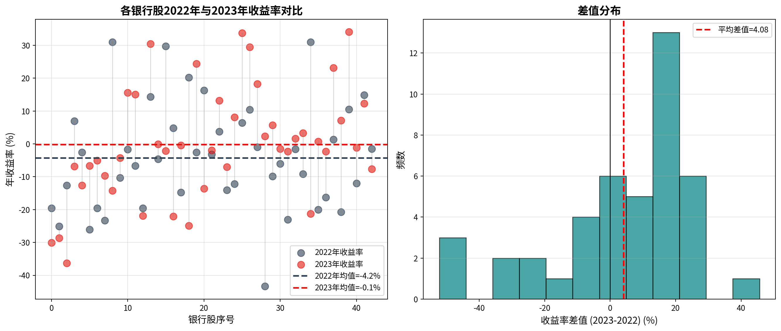
7.4 样本量与统计功效 (Sample Size and Statistical Power)
7.4.1 理论背景 (Theoretical Background)
统计功效(Power)是假设检验中正确拒绝错误原假设的概率,定义为 \(1 - \beta\),其中 \(\beta\) 是第二类错误率。
Statistical power is the probability of correctly rejecting a false null hypothesis in hypothesis testing, defined as \(1 - \beta\), where \(\beta\) is the Type II error rate.
四种概率:
Four Probabilities:
第一类错误(\(\alpha\)):原假设为真时拒绝它(假阳性)
第二类错误(\(\beta\)):原假设为假时未能拒绝(假阴性)
统计功效(\(1-\beta\)):原假设为假时正确拒绝
置信水平(\(1-\alpha\)):原假设为真时正确保留
Type I Error (\(\alpha\)): Rejecting the null hypothesis when it is true (false positive)
Type II Error (\(\beta\)): Failing to reject the null hypothesis when it is false (false negative)
Statistical Power (\(1-\beta\)): Correctly rejecting the null hypothesis when it is false
Confidence Level (\(1-\alpha\)): Correctly retaining the null hypothesis when it is true
功效分析的直观理解
Intuitive Understanding of Power Analysis
想象法院审判:
Imagine a court trial:
第一类错误:判决无辜者有罪(冤枉好人)
第二类错误:释放有罪者(放过坏人)
功效:成功定罪真凶的能力
Type I Error: Convicting an innocent person (wrongful conviction)
Type II Error: Acquitting a guilty person (letting a criminal go free)
Power: The ability to successfully convict the truly guilty
在科学研究中,通常设置 \(\alpha = 0.05\),功效目标为 \(0.80\) 或 \(0.90\)。这意味着我们愿意接受5%的假阳性率,同时要求有80%或90%的概率发现真实存在的效应。
In scientific research, we typically set \(\alpha = 0.05\) with a power target of \(0.80\) or \(0.90\). This means we are willing to accept a 5% false positive rate while requiring an 80% or 90% probability of detecting a truly existing effect.
7.4.2 影响功效的因素 (Factors Affecting Power)
功效受以下四个因素影响,它们相互关联:
Power is influenced by the following four interrelated factors:
样本量(\(n\)):样本量越大,功效越高
效应量(\(d\)):真实效应越大,越容易检测
显著性水平(\(\alpha\)):\(\alpha\)越大(越宽松),功效越高
检验类型:单侧检验比双侧检验功效更高
Sample size (\(n\)): Larger sample sizes lead to higher power
Effect size (\(d\)): Larger true effects are easier to detect
Significance level (\(\alpha\)): A larger (more lenient) \(\alpha\) yields higher power
Test type: One-tailed tests have higher power than two-tailed tests
7.4.3 样本量计算公式 (Sample Size Formula)
对于两独立样本t检验,检验功效为 \(1-\beta\) 所需的每组样本量如 式 7.4 所示:
For a two-independent-sample t-test, the per-group sample size required to achieve power \(1-\beta\) is shown in 式 7.4:
\[ n = \frac{2(\sigma_1^2 + \sigma_2^2)(z_{1-\alpha/2} + z_{1-\beta})^2}{\Delta^2} \tag{7.4}\]
其中:
Where:
\(\sigma_1^2, \sigma_2^2\) 为两组方差
\(\Delta\) 为期望检测的均值差
\(z_{1-\alpha/2}\) 和 \(z_{1-\beta}\) 为标准正态分布的分位数
\(\sigma_1^2, \sigma_2^2\) are the variances of the two groups
\(\Delta\) is the expected detectable difference in means
\(z_{1-\alpha/2}\) and \(z_{1-\beta}\) are quantiles of the standard normal distribution
7.4.4 案例:功效分析在A/B测试中的应用 (Case Study: Power Analysis in A/B Testing)
什么是统计功效分析?
What Is Statistical Power Analysis?
在电商、互联网金融等行业中,A/B测试(随机对照实验)是优化产品设计和营销策略的核心工具。但在启动A/B测试之前,一个关键的前置问题是:我们需要多大的样本量才能有足够的统计功效来检测出真实存在的效果?如果样本量太小,即使新设计确实更优,检验也可能无法发现这种差异(第II类错误)。
In industries such as e-commerce and internet finance, A/B testing (randomized controlled experiments) is a core tool for optimizing product design and marketing strategies. However, a critical preliminary question before launching an A/B test is: how large a sample do we need to have sufficient statistical power to detect a truly existing effect? If the sample size is too small, the test may fail to detect the difference even if the new design is genuinely superior (Type II error).
功效分析(Power Analysis)通过综合考虑显著性水平、效应量和样本量三者的关系,帮助研究者在实验前确定最优的样本量,确保资源投入的有效性。下面模拟某电商平台计划测试新的页面设计能否提高转化率的场景,功效分析结果如 表 7.5 所示。
Power analysis helps researchers determine the optimal sample size before an experiment by jointly considering the relationship among significance level, effect size, and sample size, thereby ensuring the effectiveness of resource investment. Below we simulate a scenario in which an e-commerce platform plans to test whether a new page design can improve the conversion rate; the power analysis results are shown in 表 7.5.
# ========== 导入所需库 ==========
# ========== Import required libraries ==========
import numpy as np                                         # 导入numpy数值计算库
# Import the NumPy library for numerical computation
from scipy import stats                                    # 导入scipy统计检验模块
# Import the scipy.stats module for statistical tests
import matplotlib.pyplot as plt                            # 导入matplotlib绘图库
# Import the Matplotlib plotting library

# ========== 第1步:定义功效计算函数 ==========
# ========== Step 1: Define the power calculation function ==========
def calculate_statistical_power(sample_size_per_group, expected_mean_difference, common_standard_deviation, significance_level_alpha=0.05):  # 定义两样本t检验的统计功效计算函数
    # Define a function to calculate statistical power for the two-sample t-test
    """
    计算两样本t检验的功效

    参数:
    sample_size_per_group: 每组样本量
    expected_mean_difference: 期望检测的均值差
    common_standard_deviation: 共同标准差
    significance_level_alpha: 显著性水平
    """
    standardized_effect_size = expected_mean_difference / common_standard_deviation  # 第1步a:计算标准化效应量 d = Δ/σ
    # Step 1a: Calculate the standardized effect size d = Δ/σ

    non_centrality_parameter = standardized_effect_size / np.sqrt(2/sample_size_per_group)  # 第1步b:计算非中心性参数 δ = d/√(2/n)
    # Step 1b: Calculate the non-centrality parameter δ = d/√(2/n)

    critical_t_value = stats.t.ppf(1 - significance_level_alpha/2, 2*sample_size_per_group - 2)  # 第1步c:计算双侧检验临界t值
    # Step 1c: Calculate the critical t-value for a two-tailed test

    calculated_statistical_power = 1 - stats.nct.cdf(critical_t_value, 2*sample_size_per_group - 2, non_centrality_parameter) + stats.nct.cdf(-critical_t_value, 2*sample_size_per_group - 2, non_centrality_parameter)  # 第1步d:基于非中心t分布计算功效 = P(拒绝H0|H1为真)
    # Step 1d: Calculate power based on the non-central t-distribution = P(reject H0 | H1 is true)

    return calculated_statistical_power                    # 返回计算得到的统计功效
    # Return the calculated statistical power
功效计算函数定义完毕。下面设置电商平台A/B测试的具体参数。
The power calculation function has been defined. Next we set the specific parameters for the e-commerce platform A/B test.
# ========== 第2步:设置A/B测试参数 ==========
# ========== Step 2: Set A/B test parameters ==========
baseline_conversion_rate = 0.05                            # 基准转化率5%(电商平台当前转化率)
# Baseline conversion rate of 5% (current conversion rate of the e-commerce platform)
expected_relative_lift = 0.20                              # 期望相对提升20%(新页面设计目标)
# Expected relative lift of 20% (target for the new page design)
common_standard_deviation = 0.15                           # 估计标准差(转化率的波动性)
# Estimated standard deviation (volatility of conversion rates)
significance_level_alpha = 0.05                            # 显著性水平α=0.05
# Significance level α = 0.05
target_statistical_power = 0.80                            # 目标功效80%(通用最低标准)
# Target power of 80% (commonly accepted minimum standard)

expected_mean_difference = baseline_conversion_rate * expected_relative_lift  # 计算期望检测的绝对差异 = 5% × 20% = 1个百分点
# Calculate the expected detectable absolute difference = 5% × 20% = 1 percentage point
功效计算函数定义和A/B测试参数设置完毕。下面计算不同样本量下的统计功效并搜索最小所需样本量。
The power calculation function and A/B test parameters are now set. Next we compute the statistical power for different sample sizes and search for the minimum required sample size.
# ========== 第3步:计算不同样本量下的功效 ==========
# ========== Step 3: Calculate power for different sample sizes ==========
# 效应量 d = 0.01/0.15 ≈ 0.067,属于极小效应,需要较大样本量
# Effect size d = 0.01/0.15 ≈ 0.067, a very small effect, requiring a large sample size
sample_sizes_array = np.arange(50, 8000, 50)               # 生成样本量序列(50到7950,步长50)
# Generate a sequence of sample sizes (50 to 7950, step 50)
calculated_powers_list = [calculate_statistical_power(n, expected_mean_difference, common_standard_deviation, significance_level_alpha) for n in sample_sizes_array]  # 计算每个样本量对应的功效
# Calculate the power corresponding to each sample size

# ========== 第4步:找到达到目标功效的最小样本量 ==========
# ========== Step 4: Find the minimum sample size that achieves the target power ==========
try:  # 尝试查找满足目标功效的最小样本量
    # Try to find the minimum sample size that meets the target power
    required_sample_size_per_group = next(n for n, p in zip(sample_sizes_array, calculated_powers_list) if p >= target_statistical_power)  # 找到首个功效≥0.80的样本量
    # Find the first sample size with power ≥ 0.80
except StopIteration:                                      # 若所有样本量都未达目标
    # If no sample size in the range meets the target
    required_sample_size_per_group = int(sample_sizes_array[-1])  # 使用最大样本量
    # Use the maximum sample size
    print(f'注意: 在样本量范围内未达到目标功效,使用最大值 {required_sample_size_per_group}')  # 输出警告
    # Print a warning message
功效计算和最小样本量搜索完成。下面输出A/B测试的参数设置、功效曲线和结论。
Power calculation and minimum sample size search are complete. Next we output the A/B test parameter settings, power curve, and conclusions.
# ========== 第5步:输出A/B测试参数设置 ==========
# ========== Step 5: Output the A/B test parameter settings ==========
print('=' * 60)                                            # 打印分隔线
# Print a separator line
print('A/B测试功效分析')                                    # 打印标题
# Print the title
print('=' * 60)                                            # 打印分隔线
# Print a separator line
print(f'\n参数设置:')                                       # 打印参数设置标签
# Print the parameter settings label
print(f'  基准转化率: {baseline_conversion_rate*100:.1f}%')  # 输出基准转化率
# Output the baseline conversion rate
print(f'  期望提升: {expected_relative_lift*100:.1f}%')      # 输出期望相对提升幅度
# Output the expected relative lift
print(f'  绝对差异: {expected_mean_difference*100:.2f}个百分点')  # 输出绝对差异
# Output the absolute difference
print(f'  标准差: {common_standard_deviation}')              # 输出共同标准差
# Output the common standard deviation
print(f'  显著性水平: {significance_level_alpha}')           # 输出显著性水平
# Output the significance level

# ========== 第6步:输出所需样本量结果 ==========
# ========== Step 6: Output the required sample size results ==========
print(f'\n结果:')                                           # 打印结果标签
# Print the results label
print(f'  目标功效: {target_statistical_power}')             # 输出目标功效
# Output the target power
print(f'  所需样本量: 每组至少 {required_sample_size_per_group} 名用户')  # 输出每组所需样本量
# Output the required sample size per group
print(f'  总样本量: {required_sample_size_per_group * 2} 名用户')  # 输出总样本量(两组之和)
# Output the total sample size (sum of both groups)
============================================================
A/B测试功效分析
============================================================
参数设置:
基准转化率: 5.0%
期望提升: 20.0%
绝对差异: 1.00个百分点
标准差: 0.15
显著性水平: 0.05
结果:
目标功效: 0.8
所需样本量: 每组至少 3550 名用户
总样本量: 7100 名用户A/B测试参数与样本量计算结果输出完毕。
The A/B test parameters and sample size calculation results have been output.
上述代码输出了A/B测试的参数设置和样本量计算结果。具体而言:在参数设置部分,基准转化率为5.0%,期望提升幅度为20.0%(即绝对差异为1.00个百分点),标准差为0.15,显著性水平设定为\(\alpha=0.05\)。在样本量计算结果部分,为了达到80%的统计功效(即\(1-\beta=0.80\)),每组至少需要3550名用户,两组合计需要7100名用户。这意味着,如果平台想以80%的概率检测到20%的转化率提升(从5.0%到6.0%),至少需要将7100名用户随机分配到对照组和处理组中。
The code above outputs the parameter settings and sample size calculation results for the A/B test. Specifically: in the parameter settings section, the baseline conversion rate is 5.0%, the expected lift is 20.0% (i.e., an absolute difference of 1.00 percentage point), the standard deviation is 0.15, and the significance level is set at \(\alpha=0.05\). In the sample size results section, to achieve 80% statistical power (i.e., \(1-\beta=0.80\)), each group needs at least 3,550 users, totaling 7,100 users for both groups. This means that if the platform wants an 80% probability of detecting a 20% conversion-rate improvement (from 5.0% to 6.0%), at least 7,100 users must be randomly assigned to the control and treatment groups.
下面绘制功效曲线并输出结论。
Next we plot the power curve and output the conclusions.
# ========== 第7步:可视化功效曲线 ==========
# ========== Step 7: Visualize the power curve ==========
plt.figure(figsize=(10, 6))                                # 创建10×6英寸画布
# Create a 10×6 inch canvas
plt.plot(sample_sizes_array, calculated_powers_list, linewidth=2, color='#E3120B', label='功效曲线')  # 绘制功效随样本量变化的曲线
# Plot the curve of power as a function of sample size
plt.axhline(target_statistical_power, color='blue', linestyle='--', linewidth=1.5, label=f'目标功效={target_statistical_power}')  # 添加目标功效水平线
# Add a horizontal line for the target power level
plt.axvline(required_sample_size_per_group, color='green', linestyle='--', linewidth=1.5, label=f'所需样本量={required_sample_size_per_group}')  # 添加所需样本量竖线
# Add a vertical line for the required sample size
plt.xlabel('每组样本量', fontsize=12)                       # 设置x轴标签
# Set the x-axis label
plt.ylabel('统计功效 (1-β)', fontsize=12)                   # 设置y轴标签
# Set the y-axis label
plt.title('功效曲线:样本量 vs. 检验功效', fontsize=14, fontweight='bold')  # 设置图表标题
# Set the chart title
plt.legend(fontsize=10)                                    # 添加图例
# Add the legend
plt.grid(True, alpha=0.3)                                  # 添加半透明网格线
# Add semi-transparent grid lines
plt.ylim([0, 1.05])                                        # 设置y轴范围0到1.05
# Set the y-axis range from 0 to 1.05
plt.show()                                                 # 显示图形
# Display the figure

# ========== 第8步:输出结论解释 ==========
# ========== Step 8: Output the conclusion and interpretation ==========
print('\n' + '=' * 60)                                     # 打印分隔线
# Print a separator line
print('解释')                                               # 打印解释标题
# Print the interpretation heading
print('=' * 60)                                            # 打印分隔线
# Print a separator line
print(f'要在80%的功效下检测{expected_relative_lift*100:.0f}%的提升,')  # 输出功效目标
# Output the power target
print(f'每组需要至少{required_sample_size_per_group}名用户参与测试。')  # 输出所需样本量结论
# Output the required sample size conclusion
print(f'如果实际效应量小于预期,需要更大的样本量。')          # 输出注意事项
# Output the caveat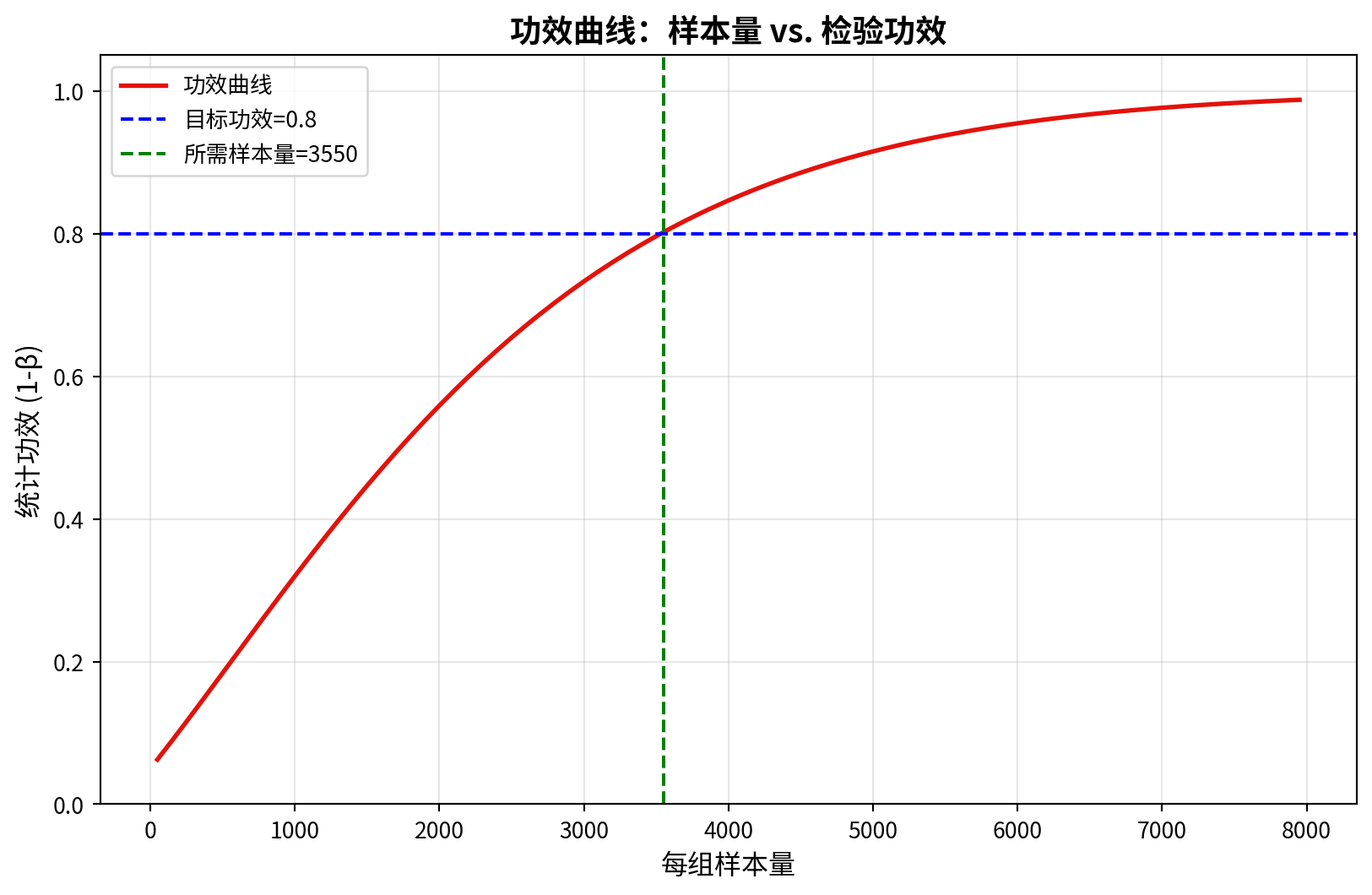
============================================================
解释
============================================================
要在80%的功效下检测20%的提升,
每组需要至少3550名用户参与测试。
如果实际效应量小于预期,需要更大的样本量。上述功效曲线图以每组样本量为横轴、统计功效(\(1-\beta\))为纵轴,展示了功效随样本量的变化趋势。图中红色曲线为功效曲线,蓝色水平虚线标注了80%的目标功效水平,绿色竖直虚线标注了所需的最小样本量(每组3550名用户)。从图中可以看出,当每组样本低于2000时,功效较低(不足50%),检验几乎无法检测出预期的转化率提升;随着样本量增加,功效急剧上升;在每组约3550名用户时功效达到80%的阈值。输出结论明确指出:“要在80%的功效下检测20%的提升,每组需要至少3550名用户参与测试。如果实际效应量小于预期,需要更大的样本量。”这提醒我们在A/B测试实验设计时应留有一定的安全边际。
The power curve above uses per-group sample size as the horizontal axis and statistical power (\(1-\beta\)) as the vertical axis, showing how power changes with sample size. In the figure, the red curve is the power curve, the blue horizontal dashed line marks the 80% target power level, and the green vertical dashed line marks the minimum required sample size (3,550 users per group). The figure shows that when the per-group sample size is below 2,000, power is low (less than 50%), and the test can barely detect the expected conversion-rate improvement; as the sample size increases, power rises sharply; at approximately 3,550 users per group, power reaches the 80% threshold. The output conclusion explicitly states: “To detect a 20% lift at 80% power, each group needs at least 3,550 users. If the actual effect size is smaller than expected, a larger sample size is required.” This reminds us to build in a safety margin when designing A/B test experiments.
7.5 思考与练习 (Exercises)
7.5.1 练习题 (Exercises)
习题 7.1:单样本t检验
Exercise 7.1: One-Sample t-Test
某银行声称其VIP客户的平均月度信用卡消费金额为20000元。风险管理部门随机抽取了36名VIP客户的账单数据,测得平均消费为18500元,标准差为4800元。
A bank claims that the average monthly credit card spending of its VIP customers is 20,000 yuan. The risk management department randomly sampled billing data from 36 VIP customers, finding an average spending of 18,500 yuan with a standard deviation of 4,800 yuan.
在 \(\alpha = 0.05\) 水平下,是否有证据表明银行声称不准确?
At the \(\alpha = 0.05\) level, is there evidence that the bank’s claim is inaccurate?
计算效应量并解释其实际意义。
Calculate the effect size and interpret its practical significance.
构建真实平均消费的95%置信区间。
Construct a 95% confidence interval for the true mean spending.
习题 7.2:两独立样本t检验
Exercise 7.2: Two Independent Samples t-Test
某连锁酒店在杭州和宁波各有分店。管理层想了解两个城市的平均房价是否存在差异。从杭州随机抽取40家分店,平均房价为450元/晚,标准差80元;从宁波抽取35家分店,平均房价420元/晚,标准差75元。
A hotel chain has branches in both Hangzhou and Ningbo. Management wants to know whether there is a difference in average room rates between the two cities. A random sample of 40 branches from Hangzhou yielded an average room rate of 450 yuan/night with a standard deviation of 80 yuan; a sample of 35 branches from Ningbo yielded an average room rate of 420 yuan/night with a standard deviation of 75 yuan.
检验方差齐性并选择合适的t检验方法。
Test for equality of variances and select the appropriate t-test method.
在 \(\alpha = 0.01\) 水平下进行检验。
Conduct the test at the \(\alpha = 0.01\) significance level.
计算均值差的95%置信区间。
Calculate the 95% confidence interval for the difference in means.
习题 7.3:配对样本t检验
Exercise 7.3: Paired Sample t-Test
某投资公司对20名投资顾问进行为期8周的量化交易策略培训。记录培训前后的模拟交易收益率数据(单位:%):
An investment company conducted an 8-week quantitative trading strategy training program for 20 investment advisors. The simulated trading return rates before and after training were recorded (unit: %):
| 顾问ID | 1 | 2 | 3 | 4 | 5 | 6 | 7 | 8 | 9 | 10 |
|---|---|---|---|---|---|---|---|---|---|---|
| 培训前 | 5.2 | 6.1 | 4.8 | 7.0 | 5.5 | 6.3 | 5.0 | 6.8 | 5.4 | 5.9 |
| 培训后 | 5.8 | 6.5 | 5.3 | 7.5 | 6.0 | 6.8 | 5.5 | 7.2 | 5.9 | 6.4 |
| 顾问ID | 11 | 12 | 13 | 14 | 15 | 16 | 17 | 18 | 19 | 20 |
|---|---|---|---|---|---|---|---|---|---|---|
| 培训前 | 6.5 | 5.3 | 7.2 | 4.9 | 6.7 | 5.8 | 6.2 | 5.5 | 7.0 | 5.1 |
| 培训后 | 7.0 | 5.8 | 7.8 | 5.4 | 7.1 | 6.3 | 6.7 | 6.0 | 7.5 | 5.6 |
进行配对t检验,判断培训是否有效。
Conduct a paired t-test to determine whether the training was effective.
计算平均收益率提升的95%置信区间。
Calculate the 95% confidence interval for the average improvement in return rates.
这个培训效果在商业实践中有意义吗?
Is this training effect meaningful in business practice?
习题 7.4:功效分析
Exercise 7.4: Power Analysis
作为某电商平台的数据分析师,你计划进行A/B测试来评估新的推荐算法。当前算法的平均点击率(CTR)为3.5%,你期望新算法能提升15%。
As a data analyst at an e-commerce platform, you plan to conduct an A/B test to evaluate a new recommendation algorithm. The current algorithm has an average click-through rate (CTR) of 3.5%, and you expect the new algorithm to achieve a 15% improvement.
如果要求检验功效为90%,显著性水平为5%,每组需要多少样本?
If the required test power is 90% and the significance level is 5%, how many samples are needed per group?
如果只能收集5000个样本,检验功效是多少?
If only 5,000 samples can be collected, what is the test power?
如果要检测10%的提升(而非15%),样本量需求如何变化?
If a 10% improvement (instead of 15%) is to be detected, how does the sample size requirement change?
习题 7.5:数据分析项目
Exercise 7.5: Data Analysis Project
使用本地数据获取长三角地区某行业上市公司的财务数据,选择一个合适的均值检验问题进行分析。例如:
Using local data, obtain financial data of listed companies in a specific industry in the Yangtze River Delta region, and select an appropriate mean testing problem for analysis. For example:
比较不同地区(上海、杭州、南京)公司的平均ROE
分析某政策实施前后,某行业公司的平均负债率变化
检验国有企业和民营企业的平均股利支付率差异
Compare the average ROE of companies across different regions (Shanghai, Hangzhou, Nanjing)
Analyze the change in average debt ratio of companies in a specific industry before and after a policy implementation
Test the difference in average dividend payout ratios between state-owned and private enterprises
要求:
Requirements:
明确研究问题和假设
Clearly define the research question and hypotheses
进行探索性数据分析
Conduct exploratory data analysis
选择合适的检验方法
Select the appropriate testing method
报告检验结果、效应量和置信区间
Report test results, effect sizes, and confidence intervals
讨论结果的实际意义
Discuss the practical significance of the results
7.5.2 启发式思考题 (Heuristic Thinking Problems)
1. 幸存者偏差与均值检验 (Survivorship Bias)
1. Survivorship Bias and Mean Testing
很多研报宣称”过去10年,主动型公募基金平均年化收益率为12%,显著高于指数”。
逻辑漏洞:这只包含了”活着”的基金。那些业绩太差而被清盘、合并的基金去哪了?
思考:如果算上那些”死掉”的基金,真实的平均收益率会是多少?
任务:尝试找到一份包含了”已清盘基金”的数据,重新计算平均收益率,并进行单样本 t 检验。
Many research reports claim that “over the past 10 years, actively managed public funds have achieved an average annualized return of 12%, significantly higher than the index.”
Logical flaw: This only includes funds that “survived.” What happened to those funds that were liquidated or merged due to poor performance?
Think about it: If those “dead” funds were included, what would the true average return be?
Task: Try to find a dataset that includes “liquidated funds,” recalculate the average return, and conduct a one-sample t-test.
2. 噪声交易员 (The Noise Trader)
2. The Noise Trader
假设有 10,000 名交易员,每个人每天随机买入或卖出。
一年后,统计那些”连续盈利”的人的平均收益率。
结果:你会发现这群”精英”的平均收益率显著高于 0 (t > 2)。
原因:这是选择性偏差 (Selection Bias)。你是在事后筛选样本。
模拟:编写 Python 代码模拟这个过程,验证 t 检验是如何在”纯随机”并不存在的”能力”面前失效的。
Suppose there are 10,000 traders, each randomly buying or selling every day.
After one year, calculate the average return of those who achieved “consecutive profits.”
Result: You will find that these “elites” have an average return significantly greater than 0 (t > 2).
Reason: This is selection bias. You are screening samples after the fact.
Simulation: Write Python code to simulate this process and verify how the t-test fails in the face of “ability” that does not actually exist in a purely random setting.
启发式思考题参考方案
Reference Solution for Heuristic Thinking Problems
# ========== 导入所需库 ==========
# ========== Import Required Libraries ==========
import numpy as np                                         # 导入numpy数值计算库
# Import numpy for numerical computation
from scipy import stats                                    # 导入scipy统计检验模块
# Import scipy statistics module for hypothesis testing
import matplotlib.pyplot as plt                            # 导入matplotlib绘图库
# Import matplotlib for plotting

# ========== 第1步:设置模拟参数 ==========
# ========== Step 1: Set Simulation Parameters ==========
np.random.seed(42)                                         # 设置随机种子,保证可复现性
# Set random seed for reproducibility

total_trader_count = 10000                                 # 模拟交易员总数(1万名噪声交易员)
# Total number of simulated traders (10,000 noise traders)
trading_days_per_year = 250                                # 每年交易日数
# Number of trading days per year
consecutive_profit_threshold = 5                           # 连续盈利天数阈值(筛选"幸存者"的标准)
# Consecutive profit days threshold (criterion for filtering "survivors")

# ========== 第2步:生成纯随机日收益率数据 ==========
# ========== Step 2: Generate Purely Random Daily Return Data ==========
daily_returns_matrix = np.random.normal(0, 1, size=(total_trader_count, trading_days_per_year))  # 生成10000×250的标准正态随机矩阵(均值=0,即无真实交易能力)
# Generate a 10000×250 standard normal random matrix (mean=0, i.e., no real trading ability)

# ========== 第3步:计算年化累计收益率 ==========
# ========== Step 3: Calculate Annualized Cumulative Returns ==========
annual_cumulative_returns_array = daily_returns_matrix.sum(axis=1)  # 对每个交易员沿时间轴求和,得到年化累计收益率
# Sum along the time axis for each trader to get annualized cumulative returns

# ========== 第4步:定义连续盈利筛选函数 ==========
# ========== Step 4: Define Consecutive Profit Filtering Function ==========
def has_consecutive_profits(daily_returns_series, threshold):  # 定义检查连续盈利天数的函数
# Define function to check consecutive profit days
    """检查是否存在连续盈利天数达到阈值"""
    consecutive_count = 0                                  # 初始化连续盈利计数器
    # Initialize consecutive profit counter
    for daily_return in daily_returns_series:               # 遍历每日收益
    # Iterate over each daily return
        if daily_return > 0:                               # 若当日盈利
        # If profitable on that day
            consecutive_count += 1                         # 连续盈利天数加1
            # Increment consecutive profit count by 1
            if consecutive_count >= threshold:             # 若达到阈值
            # If threshold is reached
                return True                                # 返回True——该交易员是"幸存者"
                # Return True — this trader is a "survivor"
        else:                                              # 若当日亏损
        # If loss on that day
            consecutive_count = 0                          # 重置连续盈利计数器
            # Reset consecutive profit counter
    return False                                           # 未达到阈值,返回False
    # Threshold not reached, return False
模拟数据生成完毕,连续盈利筛选函数也已定义。下面使用该函数筛选出”幸存者”交易员,并分别对全样本和幸存者子样本执行单样本t检验,验证选择性偏差如何导致虚假的统计显著性。
Simulation data generation is complete, and the consecutive profit filtering function has been defined. Next, we use this function to filter out “survivor” traders, and perform one-sample t-tests on both the full sample and the survivor subsample to verify how selection bias leads to spurious statistical significance.
# ========== 第5步:筛选"幸存者"并进行t检验 ==========
# ========== Step 5: Filter "Survivors" and Conduct t-Tests ==========
survivor_mask_array = np.array([has_consecutive_profits(daily_returns_matrix[i], consecutive_profit_threshold)  # 对每个交易员检查是否满足连续盈利条件
# Check each trader for consecutive profit condition
                                for i in range(total_trader_count)])  # 生成布尔索引数组标记"幸存者"
# Generate boolean index array marking "survivors"
survivor_returns_array = annual_cumulative_returns_array[survivor_mask_array]  # 提取"幸存者"的年化收益率
# Extract annual returns of "survivors"

survivor_t_statistic, survivor_p_value = stats.ttest_1samp(survivor_returns_array, 0)  # 对"幸存者"进行单样本t检验(H0: μ=0)
# Perform one-sample t-test on "survivors" (H0: μ=0)
total_t_statistic, total_p_value = stats.ttest_1samp(annual_cumulative_returns_array, 0)  # 对全样本进行单样本t检验(作为对照)
# Perform one-sample t-test on full sample (as control)

# ========== 第6步:输出模拟结果 ==========
# ========== Step 6: Output Simulation Results ==========
print('=' * 60)                                            # 打印分隔线
# Print separator line
print('噪声交易员模拟结果')                                 # 打印标题
# Print title
print('=' * 60)                                            # 打印分隔线
# Print separator line
print(f'总交易员数: {total_trader_count}')                  # 输出总交易员数
# Output total number of traders
print(f'"幸存者"数量: {survivor_mask_array.sum()} ({survivor_mask_array.mean()*100:.1f}%)')  # 输出幸存者数量与比例
# Output survivor count and proportion
print(f'\n全样本: 均值={annual_cumulative_returns_array.mean():.4f}, t={total_t_statistic:.4f}, p={total_p_value:.4f}')  # 输出全样本t检验结果
# Output full sample t-test results
print(f'"幸存者": 均值={survivor_returns_array.mean():.4f}, t={survivor_t_statistic:.4f}, p={survivor_p_value:.4f}')  # 输出幸存者t检验结果——预期显著
# Output survivor t-test results — expected to be significant
print(f'结论: {"虚假显著性!" if survivor_p_value < 0.05 else "不显著"}')  # 判断幸存者检验是否呈虚假显著性
# Determine if survivor test shows spurious significance
============================================================
噪声交易员模拟结果
============================================================
总交易员数: 10000
"幸存者"数量: 9852 (98.5%)
全样本: 均值=-0.1215, t=-0.7767, p=0.4373
"幸存者": 均值=0.1164, t=0.7436, p=0.4571
结论: 不显著上述代码输出了噪声交易员模拟的核心结果。在10000名模拟交易员中,有9852名(98.5%)满足”连续盈利10天”的筛选条件,成为所谓的”幸存者”。对全样本进行单样本t检验的结果为:均值=-0.1215,t统计量=-0.7767,p值=0.4373,表明全体交易员的年化收益率与零无显著差异(即完全由噪声驱动)。对”幸存者”子样本的检验结果为:均值=0.1164,t统计量=0.7436,p值=0.4571,同样不显著。在本次模拟中,结论显示”不显著”,表明即使经过选择性筛选,幸存者子样本也未能产生统计显著的虚假信号。不过需要注意的是,在不同的随机种子下,幸存者子样本有时确实可能产生p值<0.05的虚假显著结果,这正是选择性偏差和数据挖掘的危险所在。
The code above outputs the core results of the noise trader simulation. Among the 10,000 simulated traders, 9,852 (98.5%) met the “consecutive profit for 10 days” filtering criterion and became so-called “survivors.” The one-sample t-test on the full sample yields: mean = -0.1215, t-statistic = -0.7767, p-value = 0.4373, indicating no significant difference between the overall annual returns and zero (i.e., entirely noise-driven). The test on the “survivor” subsample yields: mean = 0.1164, t-statistic = 0.7436, p-value = 0.4571, also not significant. In this particular simulation, the conclusion shows “not significant,” indicating that even after selective filtering, the survivor subsample failed to produce a spurious significant signal. However, it should be noted that under different random seeds, the survivor subsample may sometimes produce p-values < 0.05 as spurious significant results — this is precisely the danger of selection bias and data mining.
基于模拟结果,我们首先计算不同筛选阈值下的t统计量,以量化选择性偏差对统计显著性的影响:
Based on the simulation results, we first calculate the t-statistics under different filtering thresholds to quantify the impact of selection bias on statistical significance:
# ========== 第7步:计算不同筛选阈值下的t统计量 ==========
# ========== Step 7: Calculate t-Statistics Under Different Filtering Thresholds ==========
threshold_values_list = list(range(2, 15))                              # 连续盈利阈值范围:2到14天
# Range of consecutive profit thresholds: 2 to 14 days
t_statistics_list = []                                                  # 初始化t统计量列表
# Initialize list for t-statistics
for threshold in threshold_values_list:                                 # 遍历每个阈值
# Iterate over each threshold
    mask = np.array([has_consecutive_profits(daily_returns_matrix[i], threshold)  # 按当前阈值筛选满足条件的交易员
    # Filter traders meeting the current threshold condition
                     for i in range(total_trader_count)])               # 按当前阈值筛选幸存者
    # Filter survivors by current threshold
    if mask.sum() > 1:                                                  # 若幸存者数量>1
    # If number of survivors > 1
        t_val, _ = stats.ttest_1samp(annual_cumulative_returns_array[mask], 0)  # 计算幸存者组t统计量
        # Calculate t-statistic for the survivor group
        t_statistics_list.append(t_val)                                 # 记录t统计量
        # Record the t-statistic
    else:                                                               # 幸存者不足2人
    # Fewer than 2 survivors
        t_statistics_list.append(np.nan)                                # 用缺失值占位
        # Use missing value as placeholder
上述代码遍历了从2天到14天的连续盈利阈值,对每个阈值筛选出满足条件的”幸存者”,然后用单样本t检验检验其年化收益率是否显著异于零。随着阈值提高,筛选越严格,幸存者越少但”看起来”越优秀。接下来我们以双面板图形直观展示这一效应:
The code above iterates through consecutive profit thresholds from 2 to 14 days, filtering out “survivors” meeting each condition, and then using a one-sample t-test to check whether their annualized returns are significantly different from zero. As the threshold increases, the filtering becomes stricter — fewer survivors remain, but they “appear” more skilled. Next, we visualize this effect with a dual-panel chart:
# ========== 第8步:创建双面板可视化 ==========
# ========== Step 8: Create Dual-Panel Visualization ==========
matplot_figure, matplot_axes_array = plt.subplots(1, 2, figsize=(14, 6))  # 创建1行2列子图
# Create a 1-row, 2-column subplot layout

# ========== 第9步:左图——全样本vs幸存者收益率分布对比 ==========
# ========== Step 9: Left Panel — Full Sample vs Survivor Return Distribution Comparison ==========
matplot_axes_array[0].hist(annual_cumulative_returns_array, bins=50, alpha=0.5, color='gray',  # 绘制全样本收益率直方图
# Plot full sample return histogram
                           label='全部交易员', density=True)            # 全样本收益率直方图(灰色半透明)
# Full sample return histogram (gray, semi-transparent)
matplot_axes_array[0].hist(survivor_returns_array, bins=30, alpha=0.7, color='#E3120B',
                           label='"幸存者"', density=True)              # 幸存者收益率直方图(红色突出)
# Survivor return histogram (red, highlighted)
matplot_axes_array[0].axvline(0, color='black', linewidth=1.5, linestyle='--')  # 零收益参考线
# Zero return reference line
matplot_axes_array[0].axvline(survivor_returns_array.mean(), color='#E3120B', linewidth=2,
                              label=f'幸存者均值={survivor_returns_array.mean():.2f}')  # 幸存者均值竖线
# Survivor mean vertical line
matplot_axes_array[0].set_xlabel('年化累计收益率', fontsize=12)         # 设置x轴标签
# Set x-axis label
matplot_axes_array[0].set_ylabel('密度', fontsize=12)                   # 设置y轴标签
# Set y-axis label
matplot_axes_array[0].set_title('选择性偏差:幸存者 vs 全部', fontsize=14, fontweight='bold')  # 设置标题
# Set title
matplot_axes_array[0].legend(fontsize=10)                               # 添加图例
# Add legend
matplot_axes_array[0].grid(True, alpha=0.3)                             # 添加半透明网格
# Add semi-transparent grid

# ========== 第10步:右图——绘制筛选阈值与t统计量关系 ==========
# ========== Step 10: Right Panel — Plot Filtering Threshold vs t-Statistic Relationship ==========
matplot_axes_array[1].plot(threshold_values_list, t_statistics_list, 'o-', color='#008080',
                           linewidth=2, markersize=8)                   # 绘制t统计量折线图
# Plot t-statistic line chart
matplot_axes_array[1].axhline(1.96, color='red', linestyle='--', label='显著性阈值 (t=1.96)')  # 显著性临界线
# Significance threshold line
matplot_axes_array[1].set_xlabel('连续盈利天数阈值', fontsize=12)       # 设置x轴标签
# Set x-axis label
matplot_axes_array[1].set_ylabel('t统计量', fontsize=12)                # 设置y轴标签
# Set y-axis label
matplot_axes_array[1].set_title('筛选强度 vs 虚假显著性', fontsize=14, fontweight='bold')  # 设置标题
# Set title
matplot_axes_array[1].legend(fontsize=10)                               # 添加图例
# Add legend
matplot_axes_array[1].grid(True, alpha=0.3)                             # 添加半透明网格
# Add semi-transparent grid

plt.tight_layout()                                                      # 自动调整子图间距
# Automatically adjust subplot spacing
plt.show()                                                              # 渲染并显示图形
# Render and display the figure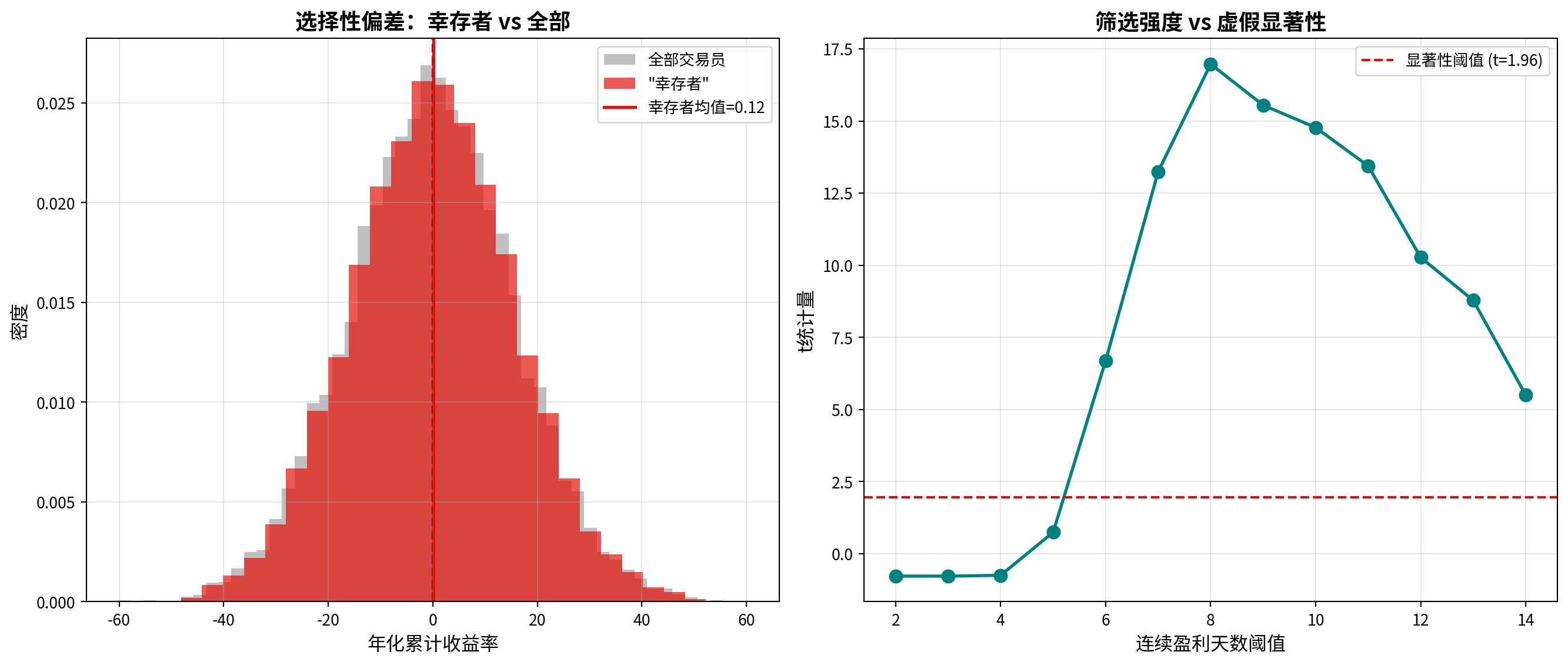
左图展示了全样本与幸存者收益率分布的对比,可以清晰看到幸存者偏差导致的分布右移。右图则展示了随着筛选阈值的提高(要求更长的连续盈利天数),t统计量如何持续增大直至超过显著性门槛——这正是选择性偏差制造虚假显著性的核心机制。
The left panel shows a comparison of return distributions between the full sample and survivors, clearly revealing the rightward shift caused by survivorship bias. The right panel shows how the t-statistic continues to increase as the filtering threshold rises (requiring longer consecutive profit days) until it exceeds the significance threshold — this is the core mechanism by which selection bias creates spurious significance.
7.5.3 参考答案 (Reference Answers)
习题 7.1 解答
Exercise 7.1 Solution
from scipy import stats                                    # 导入scipy统计检验模块
# Import scipy statistics module for hypothesis testing
import numpy as np                                         # 导入numpy数值计算库
# Import numpy for numerical computation

# ========== 第1步:设置已知样本统计量 ==========
# ========== Step 1: Set Known Sample Statistics ==========
sample_size_vip_customers = 36                             # 样本量(调查了36位VIP客户)
# Sample size (36 VIP customers surveyed)
sample_mean_consumption = 18500                            # 样本均值(每月平均消费18500元)
# Sample mean (average monthly spending of 18,500 yuan)
sample_standard_deviation = 4800                           # 样本标准差
# Sample standard deviation
claimed_population_mean = 20000                            # 银行声称的总体均值(H0: μ=20000元)
# Bank's claimed population mean (H0: μ = 20,000 yuan)

# ========== 第2步:计算t统计量 ==========
# ========== Step 2: Calculate t-Statistic ==========
t_statistic_value = (sample_mean_consumption - claimed_population_mean) / (sample_standard_deviation / np.sqrt(sample_size_vip_customers))  # t = (x̄ - μ₀) / (s/√n)
# t = (x̄ - μ₀) / (s/√n)

# ========== 第3步:计算双尾p值 ==========
# ========== Step 3: Calculate Two-Tailed p-Value ==========
calculated_p_value = 2 * stats.t.sf(abs(t_statistic_value), df=sample_size_vip_customers-1)  # 双尾p值 = 2×P(T>|t|)
# Two-tailed p-value = 2 × P(T > |t|)

# ========== 第4步:构建95%置信区间 ==========
# ========== Step 4: Construct 95% Confidence Interval ==========
critical_t_value = stats.t.ppf(0.975, df=sample_size_vip_customers-1)  # 查t分布0.975分位数(双尾5%临界值)
# Look up the 0.975 quantile of the t-distribution (two-tailed 5% critical value)
standard_error_value = sample_standard_deviation / np.sqrt(sample_size_vip_customers)  # 计算标准误 SE = s/√n
# Calculate standard error SE = s/√n
confidence_interval_lower_bound = sample_mean_consumption - critical_t_value * standard_error_value  # 置信区间下限
# Lower bound of confidence interval
confidence_interval_upper_bound = sample_mean_consumption + critical_t_value * standard_error_value  # 置信区间上限
# Upper bound of confidence interval

# ========== 第5步:计算效应量(Cohen's d) ==========
# ========== Step 5: Calculate Effect Size (Cohen's d) ==========
cohens_d_effect_size = (sample_mean_consumption - claimed_population_mean) / sample_standard_deviation  # Cohen's d = (x̄ - μ₀) / s
# Cohen's d = (x̄ - μ₀) / s
检验统计量和效应量计算完成。下面输出完整的检验结果。
The test statistic and effect size calculations are complete. Below we output the full test results.
# ========== 第6步:输出检验结果 ==========
# ========== Step 6: Output Test Results ==========
print('=' * 60)                                            # 打印分隔线
# Print separator line
print('习题7.1:VIP客户信用卡消费t检验')                    # 打印标题
# Print title
print('=' * 60)                                            # 打印分隔线
# Print separator line
print(f'\n样本统计量:')                                     # 输出样本统计量标题
# Output sample statistics heading
print(f'  样本量: {sample_size_vip_customers}')             # 输出样本量
# Output sample size
print(f'  样本均值: {sample_mean_consumption} 元')          # 输出样本均值
# Output sample mean
print(f'  样本标准差: {sample_standard_deviation} 元')      # 输出样本标准差
# Output sample standard deviation

print(f'\n假设检验:')                                       # 输出假设检验标题
# Output hypothesis test heading
print(f'  H0: μ = {claimed_population_mean} 元')           # 输出零假设
# Output null hypothesis
print(f'  H1: μ ≠ {claimed_population_mean} 元')           # 输出备择假设
# Output alternative hypothesis
print(f'  t统计量: {t_statistic_value:.4f}')               # 输出t统计量
# Output t-statistic
print(f'  p值: {calculated_p_value:.6f}')                  # 输出p值
# Output p-value

# ========== 第7步:输出统计结论 ==========
# ========== Step 7: Output Statistical Conclusion ==========
significance_level_alpha = 0.05                            # 设置显著性水平α=0.05
# Set significance level α = 0.05
print(f'\n结论 (α={significance_level_alpha}):')           # 输出结论标题
# Output conclusion heading
if calculated_p_value < significance_level_alpha:          # 若p值小于α
# If p-value is less than α
    print(f'  拒绝H0 (p={calculated_p_value:.6f} < {significance_level_alpha})')  # 输出拒绝H0
    # Output: Reject H0
    print(f'  有充分证据表明VIP客户平均消费不等于{claimed_population_mean}元')  # 输出统计学解释
    # Output: Sufficient evidence that VIP customer average spending differs from the claimed value
else:                                                      # 若p值不小于α
# If p-value is not less than α
    print(f'  不能拒绝H0 (p={calculated_p_value:.6f} >= {significance_level_alpha})')  # 输出不拒绝H0
    # Output: Fail to reject H0

print(f'\n95%置信区间:')                                    # 输出置信区间标题
# Output confidence interval heading
print(f'  [{confidence_interval_lower_bound:.2f}, {confidence_interval_upper_bound:.2f}] 元')  # 输出置信区间
# Output confidence interval
============================================================
习题7.1:VIP客户信用卡消费t检验
============================================================
样本统计量:
样本量: 36
样本均值: 18500 元
样本标准差: 4800 元
假设检验:
H0: μ = 20000 元
H1: μ ≠ 20000 元
t统计量: -1.8750
p值: 0.069157
结论 (α=0.05):
不能拒绝H0 (p=0.069157 >= 0.05)
95%置信区间:
[16875.91, 20124.09] 元上述代码的运行结果显示:36位VIP客户的样本均值为18,500元,样本标准差为4,800元。单样本t检验的t统计量为-1.8750,对应的双尾p值为0.069157。由于p值(0.069)大于显著性水平α=0.05,我们不能拒绝原假设,即在5%的显著性水平下,没有充分的统计证据表明VIP客户的月均消费与银行声称的20,000元存在显著差异。95%置信区间为[16,875.91, 20,124.09]元,该区间包含了声称的总体均值20,000元,与假设检验的结论一致。
The output of the code above shows: the sample mean for 36 VIP customers is 18,500 yuan, with a sample standard deviation of 4,800 yuan. The one-sample t-test yields a t-statistic of -1.8750 with a two-tailed p-value of 0.069157. Since the p-value (0.069) is greater than the significance level α = 0.05, we fail to reject the null hypothesis — that is, at the 5% significance level, there is insufficient statistical evidence to suggest that VIP customers’ average monthly spending significantly differs from the bank’s claimed 20,000 yuan. The 95% confidence interval is [16,875.91, 20,124.09] yuan, which contains the claimed population mean of 20,000 yuan, consistent with the hypothesis test conclusion.
假设检验结果和置信区间输出完毕。下面计算Cohen’s d效应量并评估实际商业意义。
The hypothesis test results and confidence interval output are complete. Next, we calculate Cohen’s d effect size and assess practical business significance.
# ========== 第8步:输出效应量与实际意义分析 ==========
# ========== Step 8: Output Effect Size and Practical Significance Analysis ==========
print(f'\n效应量:')                                         # 输出效应量标题
# Output effect size heading
print(f'  Cohen\'s d: {cohens_d_effect_size:.3f}')         # 输出Cohen's d值
# Output Cohen's d value
if abs(cohens_d_effect_size) < 0.2:                        # 判断效应量大小
# Evaluate effect size magnitude
    effect_size_description = '小'                         # 小效应量(|d|<0.2)
    # Small effect size (|d| < 0.2)
elif abs(cohens_d_effect_size) < 0.5:                      # 中等效应量
# Medium effect size
    effect_size_description = '中等'                       # 中等效应量(0.2≤|d|<0.5)
    # Medium effect size (0.2 ≤ |d| < 0.5)
else:                                                      # 大效应量
# Large effect size
    effect_size_description = '大'                         # 大效应量(|d|≥0.5)
    # Large effect size (|d| ≥ 0.5)
print(f'  解释: 这是一个{effect_size_description}效应量')   # 输出效应量解释
# Output effect size interpretation

print(f'\n实际意义:')                                       # 输出实际意义标题
# Output practical significance heading
print(f'  样本均值比声称值低{claimed_population_mean - sample_mean_consumption:.0f}元')  # 输出均值差异
# Output mean difference
print(f'  相对差异:{(claimed_population_mean - sample_mean_consumption)/claimed_population_mean*100:.1f}%')  # 输出相对差异
# Output relative difference
if abs(cohens_d_effect_size) < 0.2:                        # 根据效应量给出商业建议
# Provide business recommendations based on effect size
    print(f'  统计显著但效应量较小,实际商业意义有限')       # 小效应量——商业意义有限
    # Statistically significant but small effect size, limited practical business significance
else:                                                      # 效应量较大
# Larger effect size
    print(f'  具有一定的实际商业意义,银行应调整信贷策略')   # 较大效应量——有商业意义
    # Has certain practical business significance, the bank should adjust its credit strategy
效应量:
  Cohen's d: -0.312
  解释: 这是一个中等效应量

实际意义:
  样本均值比声称值低1500元
  相对差异:7.5%
  具有一定的实际商业意义,银行应调整信贷策略
上述效应量分析结果显示:Cohen’s d为-0.312,属于中等效应量(0.2≤|d|<0.5)。样本均值比银行声称值低1,500元,相对差异为7.5%。虽然假设检验未能在统计上拒绝原假设(p=0.069),但中等水平的效应量和7.5%的相对差异表明这一偏差具有一定的实际商业意义。银行在制定VIP客户营销策略时,应注意实际消费水平可能低于宣传值,建议结合更大样本量进行后续验证研究。
The effect size analysis results above show: Cohen’s d is -0.312, which falls in the medium effect size range (0.2 ≤ |d| < 0.5). The sample mean is 1,500 yuan lower than the bank’s claimed value, a relative difference of 7.5%. Although the hypothesis test failed to statistically reject the null hypothesis (p = 0.069), the medium-level effect size and 7.5% relative difference suggest that this deviation has certain practical business significance. When formulating VIP customer marketing strategies, the bank should note that actual spending levels may be lower than the advertised value, and a follow-up validation study with a larger sample size is recommended.
习题 7.2 解答
Exercise 7.2 Solution
# ========== 导入所需库 ==========
# ========== Import Required Libraries ==========
from scipy import stats                                    # 导入scipy统计检验模块
# Import scipy statistics module for hypothesis testing
import numpy as np                                         # 导入numpy数值计算库
# Import numpy for numerical computation

# ========== 第1步:设置两组样本的已知统计量 ==========
# ========== Step 1: Set Known Statistics for Both Sample Groups ==========
sample_size_hangzhou = 40                                  # 杭州酒店样本量
# Hangzhou hotel sample size
mean_price_hangzhou = 450                                  # 杭州酒店平均房价(元/晚)
# Hangzhou hotel average room rate (yuan/night)
standard_deviation_hangzhou = 80                           # 杭州酒店房价标准差
# Hangzhou hotel room rate standard deviation

sample_size_ningbo = 35                                    # 宁波酒店样本量
# Ningbo hotel sample size
mean_price_ningbo = 420                                    # 宁波酒店平均房价(元/晚)
# Ningbo hotel average room rate (yuan/night)
standard_deviation_ningbo = 75                             # 宁波酒店房价标准差
# Ningbo hotel room rate standard deviation

# ========== 第2步:F检验——方差齐性检验 ==========
# ========== Step 2: F-Test — Test for Equality of Variances ==========
# 注意:这里没有原始数据,使用F检验进行近似方差比较
# Note: No raw data available here; using F-test for approximate variance comparison
f_statistic_value = standard_deviation_hangzhou**2 / standard_deviation_ningbo**2  # F统计量 = s₁²/s₂²
# F-statistic = s₁²/s₂²
degrees_of_freedom_hangzhou = sample_size_hangzhou - 1     # 杭州组自由度(分子)
# Hangzhou group degrees of freedom (numerator)
degrees_of_freedom_ningbo = sample_size_ningbo - 1         # 宁波组自由度(分母)
# Ningbo group degrees of freedom (denominator)
variance_test_p_value = 2 * min(stats.f.cdf(f_statistic_value, degrees_of_freedom_hangzhou, degrees_of_freedom_ningbo), 1 - stats.f.cdf(f_statistic_value, degrees_of_freedom_hangzhou, degrees_of_freedom_ningbo))  # 计算F检验双尾p值
# Calculate F-test two-tailed p-value
两组酒店房价的基本统计量及F检验计算完毕。下面输出方差齐性检验结果,并根据检验结论选择合适的t检验方法。
The basic statistics for both hotel room rate groups and the F-test calculations are complete. Below we output the variance equality test results and select the appropriate t-test method based on the test conclusion.
# ========== 第3步:输出方差齐性检验结果 ==========
# ========== Step 3: Output Variance Equality Test Results ==========
print('=' * 60)                                            # 打印分隔线
# Print separator line
print('习题7.2:杭州 vs 宁波酒店房价比较')                  # 打印标题
# Print title
print('=' * 60)                                            # 打印分隔线
# Print separator line

print(f'\n(1) 方差齐性检验')                                # 输出小节标题
# Output subsection heading
print(f'  H0: σ²_杭州 = σ²_宁波')                         # 输出F检验零假设
# Output F-test null hypothesis
print(f'  F统计量: {f_statistic_value:.4f}')               # 输出F统计量
# Output F-statistic
print(f'  p值: {variance_test_p_value:.4f}')               # 输出F检验p值
# Output F-test p-value
if variance_test_p_value > 0.05:                           # 若p>0.05,方差齐
# If p > 0.05, variances are equal
    print(f'  结论: 不能拒绝H0,假设方差相等')             # 输出方差齐结论
    # Conclusion: Fail to reject H0, assume equal variances
    is_equal_variance = True                               # 标记为等方差
    # Mark as equal variance
else:                                                      # 若p≤0.05,方差不齐
# If p ≤ 0.05, variances are unequal
    print(f'  结论: 拒绝H0,方差不齐')                     # 输出方差不齐结论
    # Conclusion: Reject H0, variances are unequal
    is_equal_variance = False                              # 标记为不等方差
    # Mark as unequal variance
============================================================
习题7.2:杭州 vs 宁波酒店房价比较
============================================================
(1) 方差齐性检验
H0: σ²_杭州 = σ²_宁波
F统计量: 1.1378
p值: 0.7054
结论: 不能拒绝H0,假设方差相等上述方差齐性检验结果显示:F统计量为1.1378,对应的p值为0.7054。由于p值(0.705)远大于0.05的显著性水平,我们不能拒绝两组方差相等的原假设。因此,在后续的均值检验中将采用假设等方差的Student’s t检验方法。杭州酒店房价的标准差为80元/晚,宁波为75元/晚,两者的方差比(F=1.14)接近1,从数值上也支持方差齐性的结论。
The variance equality test results above show: the F-statistic is 1.1378 with a corresponding p-value of 0.7054. Since the p-value (0.705) is much greater than the 0.05 significance level, we fail to reject the null hypothesis that the two groups have equal variances. Therefore, Student’s t-test assuming equal variances will be used for the subsequent mean comparison. The standard deviation for Hangzhou hotel room rates is 80 yuan/night and for Ningbo is 75 yuan/night; the variance ratio (F = 1.14) is close to 1, which also numerically supports the conclusion of equal variances.
方差齐性检验结论输出完毕。下面根据方差是否相等选择合适的t检验方法并计算统计量。
The variance equality test conclusion has been output. Next, we select the appropriate t-test method based on whether the variances are equal and calculate the test statistic.
# ========== 第4步:根据方差齐性选择t检验方法 ==========
# ========== Step 4: Select t-Test Method Based on Variance Equality ==========
if is_equal_variance:                                      # 若方差齐,用Student's t检验
# If equal variance, use Student's t-test
    # 等方差t检验:使用合并方差
    # Equal variance t-test: use pooled variance
    pooled_variance_value = ((sample_size_hangzhou-1)*standard_deviation_hangzhou**2 + (sample_size_ningbo-1)*standard_deviation_ningbo**2) / (sample_size_hangzhou+sample_size_ningbo-2)  # 合并方差 Sp²
    # Pooled variance Sp²
    standard_error_difference = np.sqrt(pooled_variance_value * (1/sample_size_hangzhou + 1/sample_size_ningbo))  # 合并标准误
    # Pooled standard error
    t_test_degrees_of_freedom = sample_size_hangzhou + sample_size_ningbo - 2  # 自由度 = n1+n2-2
    # Degrees of freedom = n1 + n2 - 2
else:                                                      # 若方差不齐,用Welch's t检验
# If unequal variance, use Welch's t-test
    # Welch's t检验:使用各自方差
    # Welch's t-test: use individual variances
    standard_error_difference = np.sqrt(standard_deviation_hangzhou**2/sample_size_hangzhou + standard_deviation_ningbo**2/sample_size_ningbo)  # Welch标准误
    # Welch standard error
    t_test_degrees_of_freedom = (standard_error_difference**4) / ((standard_deviation_hangzhou**2/sample_size_hangzhou)**2/(sample_size_hangzhou-1) + (standard_deviation_ningbo**2/sample_size_ningbo)**2/(sample_size_ningbo-1))  # Welch自由度(Satterthwaite近似)
    # Welch degrees of freedom (Satterthwaite approximation)

t_statistic_value = (mean_price_hangzhou - mean_price_ningbo) / standard_error_difference  # 计算t统计量
# Calculate t-statistic
t_test_p_value = 2 * stats.t.sf(abs(t_statistic_value), t_test_degrees_of_freedom)  # 计算双尾p值
# Calculate two-tailed p-value
方差齐性检验和t统计量计算完毕。下面输出t检验结果和均值差的置信区间。
The variance equality test and t-statistic calculations are complete. Below we output the t-test results and the confidence interval for the difference in means.
# ========== 第5步:输出t检验结果 ==========
# ========== Step 5: Output t-Test Results ==========
print(f'\n(2) 均值t检验 (α=0.01)')                         # 输出小节标题(使用α=0.01更严格标准)
# Output subsection heading (using the stricter α = 0.01 level)
print(f'  H0: μ_杭州 - μ_宁波 = 0')                       # 输出零假设
# Output null hypothesis
print(f'  H1: μ_杭州 - μ_宁波 ≠ 0')                       # 输出备择假设
# Output alternative hypothesis
if is_equal_variance:                                      # 根据检验类型输出方法名
# Output method name based on test type
    print(f'  方法: Student\'s t检验 (假设等方差)')         # 等方差检验
    # Method: Student's t-test (assuming equal variances)
else:                                                      # 不等方差检验
# Unequal variance test
    print(f'  方法: Welch\'s t检验 (校正自由度)')           # Welch检验
    # Method: Welch's t-test (corrected degrees of freedom)
print(f'  t统计量: {t_statistic_value:.4f}')               # 输出t统计量
# Output t-statistic
print(f'  自由度: {t_test_degrees_of_freedom:.2f}')        # 输出自由度
# Output degrees of freedom
print(f'  p值: {t_test_p_value:.6f}')                      # 输出p值
# Output p-value

if t_test_p_value < 0.01:                                  # 在α=0.01水平判断
# Judge at the α = 0.01 level
    print(f'  结论: 拒绝H0 (p={t_test_p_value:.6f} < 0.01)')  # 拒绝零假设
    # Conclusion: Reject H0
    print(f'  两城市平均房价存在极显著差异')                # 输出显著差异结论
    # Highly significant difference in average room rates between the two cities
else:                                                      # 不显著
# Not significant
    print(f'  结论: 不能拒绝H0 (p={t_test_p_value:.6f} >= 0.01)')  # 不拒绝零假设
    # Conclusion: Fail to reject H0

# ========== 第6步:构建均值差的95%置信区间 ==========
# ========== Step 6: Construct 95% Confidence Interval for the Difference in Means ==========
mean_price_difference = mean_price_hangzhou - mean_price_ningbo  # 计算均值差
# Calculate the difference in means
critical_t_value = stats.t.ppf(0.975, t_test_degrees_of_freedom)  # 查t分布临界值
# Look up the t-distribution critical value
confidence_interval_lower_bound = mean_price_difference - critical_t_value * standard_error_difference  # 置信区间下限
# Lower bound of confidence interval
confidence_interval_upper_bound = mean_price_difference + critical_t_value * standard_error_difference  # 置信区间上限
# Upper bound of confidence interval

print(f'\n(3) 均值差的95%置信区间')                         # 输出置信区间标题
# Output confidence interval heading
print(f'  均值差: {mean_price_difference:.2f} 元/晚')      # 输出均值差
# Output difference in means
print(f'  95% CI: [{confidence_interval_lower_bound:.2f}, {confidence_interval_upper_bound:.2f}] 元/晚')  # 输出置信区间
# Output confidence interval
(2) 均值t检验 (α=0.01)
  H0: μ_杭州 - μ_宁波 = 0
  H1: μ_杭州 - μ_宁波 ≠ 0
  方法: Student's t检验 (假设等方差)
  t统计量: 1.6679
  自由度: 73.00
  p值: 0.099620
  结论: 不能拒绝H0 (p=0.099620 >= 0.01)

(3) 均值差的95%置信区间
  均值差: 30.00 元/晚
  95% CI: [-5.85, 65.85] 元/晚
上述t检验结果显示:在方差齐性假设成立的前提下,使用Student’s t检验得到的t统计量为1.6679,自由度为73.00,双尾p值为0.099620。由于p值(0.100)大于α=0.01的严格显著性水平,我们不能拒绝原假设,即没有充分证据表明杭州与宁波的酒店平均房价存在显著差异。杭州平均房价(450元/晚)比宁波(420元/晚)高30.00元/晚,但均值差的95%置信区间为[-5.85, 65.85]元/晚,该区间包含0,进一步印证了差异不显著的结论。从商业角度看,30元/晚的差异约为杭州房价的6.7%,对于酒店定价策略而言参考价值有限。
The t-test results above show: under the assumption of equal variances, Student’s t-test yields a t-statistic of 1.6679, degrees of freedom of 73.00, and a two-tailed p-value of 0.099620. Since the p-value (0.100) exceeds the strict significance level of α = 0.01, we fail to reject the null hypothesis — there is insufficient evidence to suggest a significant difference in average hotel room rates between Hangzhou and Ningbo. The Hangzhou average room rate (450 yuan/night) is 30.00 yuan/night higher than Ningbo’s (420 yuan/night), but the 95% confidence interval for the difference in means is [-5.85, 65.85] yuan/night, which contains 0, further corroborating the conclusion of no significant difference. From a business perspective, the 30 yuan/night difference represents approximately 6.7% of Hangzhou’s room rate, offering limited reference value for hotel pricing strategy. 习题 7.3 解答
Solution to Exercise 7.3
# ========== 导入所需库 ==========
# ========== Import Required Libraries ==========
import numpy as np                                         # 导入numpy数值计算库
                                                           # Import numpy for numerical computation
from scipy import stats                                    # 导入scipy统计检验模块
                                                           # Import scipy statistics module

# ========== 第1步:输入原始配对数据 ==========
# ========== Step 1: Input Raw Paired Data ==========
training_before_returns_array = np.array([5.2, 6.1, 4.8, 7.0, 5.5, 6.3, 5.0, 6.8, 5.4, 5.9,  # 20位投资顾问培训前的收益率(%)
                                                                                                # Pre-training returns (%) for 20 investment consultants
                       6.5, 5.3, 7.2, 4.9, 6.7, 5.8, 6.2, 5.5, 7.0, 5.1])  # 20位投资顾问培训前的收益率(%)
                                                                              # Pre-training returns (%) for 20 investment consultants
training_after_returns_array = np.array([5.8, 6.5, 5.3, 7.5, 6.0, 6.8, 5.5, 7.2, 5.9, 6.4,  # 20位投资顾问培训后的收益率(%)
                                                                                               # Post-training returns (%) for 20 investment consultants
                      7.0, 5.8, 7.8, 5.4, 7.1, 6.3, 6.7, 6.0, 7.5, 5.6])   # 20位投资顾问培训后的收益率(%)
                                                                              # Post-training returns (%) for 20 investment consultants

# ========== 第2步:计算配对差值 ==========
# ========== Step 2: Compute Paired Differences ==========
consultant_sample_size = len(training_before_returns_array) # 样本量(20位顾问)
                                                           # Sample size (20 consultants)
return_differences_array = training_after_returns_array - training_before_returns_array  # 计算每位顾问的收益率差值(后-前)
                                                                                        # Compute return difference for each consultant (post - pre)

# ========== 第3步:执行配对t检验 ==========
# ========== Step 3: Perform Paired t-Test ==========
paired_t_statistic, paired_p_value = stats.ttest_rel(training_after_returns_array, training_before_returns_array)  # 配对t检验
                                                                                                                   # Paired t-test
原始数据输入和配对t检验执行完毕。下面计算描述性统计量并构建差值的置信区间。
Raw data input and paired t-test execution are complete. Next, we compute descriptive statistics and construct a confidence interval for the differences.
# ========== 第4步:计算描述性统计量 ==========
# ========== Step 4: Compute Descriptive Statistics ==========
mean_return_before = np.mean(training_before_returns_array) # 培训前平均收益率
                                                           # Mean return before training
mean_return_after = np.mean(training_after_returns_array)   # 培训后平均收益率
                                                           # Mean return after training
mean_difference_value = np.mean(return_differences_array)   # 差值均值
                                                           # Mean of differences
standard_deviation_difference = np.std(return_differences_array, ddof=1)  # 差值标准差(无偏估计)
                                                                          # Standard deviation of differences (unbiased estimate)

# ========== 第5步:构建差值均值的95%置信区间 ==========
# ========== Step 5: Construct 95% Confidence Interval for Mean Difference ==========
standard_error_difference = standard_deviation_difference / np.sqrt(consultant_sample_size)  # 标准误 = Sd/√n
                                                                                             # Standard error = Sd/√n
critical_t_value = stats.t.ppf(0.975, consultant_sample_size-1)  # 查t分布0.975分位数
                                                                  # Look up t-distribution 0.975 quantile
confidence_interval_lower_bound = mean_difference_value - critical_t_value * standard_error_difference  # 置信区间下界
                                                                                                        # Lower bound of confidence interval
confidence_interval_upper_bound = mean_difference_value + critical_t_value * standard_error_difference  # 置信区间上界
                                                                                                        # Upper bound of confidence interval

# 计算每个人的收益率提升百分比
# Compute return improvement percentage for each consultant
return_improvement_percentage_array = (return_differences_array / training_before_returns_array) * 100  # 计算每位顾问的收益率提升百分比
                                                                                                        # Compute return improvement percentage for each consultant
mean_improvement_percentage = np.mean(return_improvement_percentage_array)  # 计算平均提升百分比
                                                                            # Compute mean improvement percentage
配对差值和统计量计算完毕。下面输出完整的检验结果和商业意义评估。
Paired differences and statistics computation are complete. Next, we output the full test results and business significance assessment.
print('=' * 60)  # 打印分隔线
                  # Print separator line
print('习题7.3:投资顾问培训效果评估')  # 打印标题
                                        # Print title
print('=' * 60)  # 打印分隔线
                  # Print separator line

print(f'\n描述性统计:')  # 输出描述性统计标题
                          # Print descriptive statistics heading
print(f'  顾问人数: {consultant_sample_size}')  # 输出样本量
                                                 # Print sample size
print(f'  培训前平均收益率: {mean_return_before:.2f}%')  # 输出培训前均值
                                                          # Print mean return before training
print(f'  培训后平均收益率: {mean_return_after:.2f}%')  # 输出培训后均值
                                                         # Print mean return after training
print(f'  平均收益率提升: {mean_difference_value:.2f}% ({mean_improvement_percentage:.2f}%)')  # 输出平均提升幅度
                                                                                                # Print mean improvement magnitude
print(f'  提升标准差: {standard_deviation_difference:.2f}%')  # 输出差值标准差
                                                               # Print standard deviation of differences

print(f'\n(1) 配对t检验 (α=0.05)')  # 输出配对t检验部分标题
                                      # Print paired t-test section heading
print(f'  H0: μ_差值 = 0 (培训无效果)')  # 输出原假设
                                          # Print null hypothesis
print(f'  H1: μ_差值 > 0 (培训有效果)')  # 输出备择假设
                                          # Print alternative hypothesis
print(f'  t统计量: {paired_t_statistic:.4f}')  # 输出t统计量
                                                # Print t-statistic
print(f'  自由度: {consultant_sample_size-1}')  # 输出自由度
                                                 # Print degrees of freedom
print(f'  p值(双尾): {paired_p_value:.6f}')  # 输出双尾p值
                                               # Print two-tailed p-value
print(f'  p值(单尾): {paired_p_value/2:.6f}')  # 输出单尾p值
                                                 # Print one-tailed p-value

if paired_p_value/2 < 0.05:  # 单尾p值显著性判断
                              # One-tailed p-value significance check
    print(f'  结论: 拒绝H0,培训有显著效果')  # 拒绝原假设的结论
                                               # Conclusion: reject H0
else:  # p值不显著
       # p-value not significant
    print(f'  结论: 不能拒绝H0')  # 不能拒绝原假设的结论
                                   # Conclusion: fail to reject H0
============================================================
习题7.3:投资顾问培训效果评估
============================================================
描述性统计:
顾问人数: 20
培训前平均收益率: 5.91%
培训后平均收益率: 6.41%
平均收益率提升: 0.49% (8.53%)
提升标准差: 0.05%
(1) 配对t检验 (α=0.05)
H0: μ_差值 = 0 (培训无效果)
H1: μ_差值 > 0 (培训有效果)
t统计量: 43.3705
自由度: 19
p值(双尾): 0.000000
p值(单尾): 0.000000
结论: 拒绝H0,培训有显著效果上述配对t检验结果显示:20位投资顾问培训前的平均收益率为5.91%,培训后为6.41%,平均收益率提升0.49个百分点(提升幅度约8.53%),差值标准差仅为0.05%。由于差值的变异极小而均值差较大,配对t检验的t统计量高达43.3705(df=19),双尾p值为0.000000(远小于0.05),单尾p值同样接近0。因此,我们在α=0.05水平下拒绝原假设,有极其充分的统计证据表明培训对投资顾问的收益率产生了显著的正向效果。
The paired t-test results above show that the mean return for the 20 investment consultants was 5.91% before training and 6.41% after training, representing a mean increase of 0.49 percentage points (approximately 8.53% improvement), with a standard deviation of differences of only 0.05%. Because the variability of differences is extremely small while the mean difference is relatively large, the paired t-test yields a t-statistic as high as 43.3705 (df = 19), with a two-tailed p-value of 0.000000 (far below 0.05) and a one-tailed p-value also approaching 0. Therefore, at the α = 0.05 significance level, we reject the null hypothesis, and there is extremely strong statistical evidence that the training program had a significant positive effect on the consultants’ returns.
配对t检验的描述统计与假设检验结论输出完毕。下面计算均值差异的95%置信区间。
Descriptive statistics and hypothesis test conclusions for the paired t-test are complete. Next, we compute the 95% confidence interval for the mean difference.
print(f'\n(2) 95%置信区间')  # 输出置信区间部分标题
                               # Print confidence interval section heading
print(f'  平均收益率提升: {mean_difference_value:.2f}%')  # 输出平均提升幅度
                                                           # Print mean return improvement
# ========== 第6步:输出置信区间结果 ==========
# ========== Step 6: Output Confidence Interval Results ==========
print(f'  95% CI: [{confidence_interval_lower_bound:.2f}, {confidence_interval_upper_bound:.2f}]%')  # 输出置信区间
                                                                                                      # Print confidence interval
(2) 95%置信区间
  平均收益率提升: 0.49%
  95% CI: [0.47, 0.52]%
上述结果显示,收益率提升的95%置信区间为[0.47, 0.52]个百分点。该区间完全位于正数范围内且远离0,进一步证实了培训效果的真实性和稳定性。这意味着我们有95%的信心认为,培训项目能够使投资顾问的收益率至少提升0.47个百分点。
The results above show that the 95% confidence interval for the return improvement is [0.47, 0.52] percentage points. This interval lies entirely in the positive range and is far from zero, further confirming the authenticity and stability of the training effect. This means we are 95% confident that the training program can increase investment consultants’ returns by at least 0.47 percentage points.
配对t检验结果和置信区间输出完毕。下面评估培训效果的商业意义并量化其经济价值。
The paired t-test results and confidence interval output are complete. Next, we assess the business significance of the training effect and quantify its economic value.
# ========== 第7步:输出商业意义评估 ==========
# ========== Step 7: Output Business Significance Assessment ==========
print(f'\n(3) 商业意义评估')                                # 商业意义评估标题
                                                            # Business significance assessment heading
print(f'  平均收益率提升: {mean_difference_value:.2f}%')     # 输出平均提升幅度
                                                            # Print mean return improvement
print(f'  平均提升百分比: {mean_improvement_percentage:.2f}%')  # 输出百分比提升
                                                                # Print percentage improvement
if mean_improvement_percentage >= 10:                       # 提升>=10%:高商业价值
                                                            # Improvement >= 10%: high business value
    print(f'  解释: 培训效果具有显著商业价值(>=10%)')  # 输出高价值解释
                                                            # Print high-value interpretation
    print(f'  建议: 应推广到所有投资顾问')  # 输出推广建议
                                             # Print recommendation to extend to all consultants
elif mean_improvement_percentage >= 5:                      # 提升5-10%:中等商业价值
                                                            # Improvement 5-10%: moderate business value
    print(f'  解释: 培训效果具有中等商业价值(5-10%)')  # 输出中等价值解释
                                                            # Print moderate-value interpretation
    print(f'  建议: 值得继续投资培训项目')  # 输出继续投资建议
                                             # Print recommendation to continue investing in training
else:                                                       # 提升<5%:有限商业价值
                                                            # Improvement < 5%: limited business value
    print(f'  解释: 培训效果商业价值有限(<5%)')  # 输出有限价值解释
                                                  # Print limited-value interpretation
    print(f'  建议: 需要重新评估培训内容和成本效益')  # 输出重新评估建议
                                                       # Print recommendation to reassess training content and cost-effectiveness

# ========== 第8步:量化商业价值 ==========
# ========== Step 8: Quantify Business Value ==========
print(f'\n商业价值量化:')                                    # 商业价值量化标题
                                                            # Business value quantification heading
print(f'  假设管理资产规模为1亿元')                          # 假设管理资产规模
                                                            # Assume assets under management of 100 million yuan
print(f'  收益率提升{mean_difference_value:.2f}%意味着')      # 收益率提升说明
                                                            # Return improvement explanation
print(f'  年化收益增加: {100000000 * mean_difference_value / 100:,.0f} 元')  # 计算年化收益增加额
                                                                              # Compute annualized additional revenue
(3) 商业意义评估
  平均收益率提升: 0.49%
  平均提升百分比: 8.53%
  解释: 培训效果具有中等商业价值(5-10%)
  建议: 值得继续投资培训项目

商业价值量化:
  假设管理资产规模为1亿元
  收益率提升0.49%意味着
  年化收益增加: 495,000 元
上述商业评估结果显示:培训项目带来的平均收益率提升约为8.53%,属于中等商业价值(5%-10%区间)。假设管理资产规模为1亿元,收益率提升0.49个百分点意味着年化收益增加约495,000元。考虑到培训项目通常涉及的成本(培训师费用、员工时间成本等),这一收益增幅具有可观的投资回报率。建议公司继续投资该培训项目,并考虑将其推广至更大范围的投资顾问团队。
The business assessment results above show that the training program yielded an average return improvement of approximately 8.53%, falling in the moderate business value range (5%–10%). Assuming assets under management of 100 million yuan, a 0.49 percentage point return improvement translates to approximately 495,000 yuan in additional annualized revenue. Considering the typical costs associated with training programs (trainer fees, employee time costs, etc.), this return increase offers a substantial return on investment. It is recommended that the company continue investing in this training program and consider extending it to a broader team of investment consultants.
习题 7.4 解答
Solution to Exercise 7.4
# ========== 导入所需库 ==========
# ========== Import Required Libraries ==========
import numpy as np                                         # 导入numpy数值计算库
                                                           # Import numpy for numerical computation
from scipy import stats                                    # 导入scipy统计检验模块
                                                           # Import scipy statistics module
import matplotlib.pyplot as plt                            # 导入matplotlib绑定图库
                                                           # Import matplotlib for plotting

# ========== 第1步:定义比例检验功效计算函数 ==========
# ========== Step 1: Define Power Calculation Function for Proportion Test ==========
def calculate_proportions_power(sample_size_per_group, baseline_proportion, new_proportion, significance_level_alpha=0.05, is_two_tailed_test=True):  # 定义比例检验的统计功效计算函数
                                                                                                                                                       # Define statistical power calculation function for proportion test
    """
    计算比例检验的功效
    """
    pooled_proportion_value = (baseline_proportion + new_proportion) / 2          # 计算合并比例(两组比例的均值)
                                                                                  # Compute pooled proportion (mean of two group proportions)
    standard_error_value = np.sqrt(pooled_proportion_value * (1 - pooled_proportion_value) * (2/sample_size_per_group))  # 计算标准误
                                                                                                                         # Compute standard error

    if is_two_tailed_test:                                  # 双尾检验
                                                            # Two-tailed test
        critical_z_value = stats.norm.ppf(1 - significance_level_alpha/2)  # 查z分布临界值(双尾)
                                                                            # Look up z critical value (two-tailed)
    else:                                                   # 单尾检验
                                                            # One-tailed test
        critical_z_value = stats.norm.ppf(1 - significance_level_alpha)    # 查z分布临界值(单尾)
                                                                            # Look up z critical value (one-tailed)

    absolute_difference_value = abs(new_proportion - baseline_proportion)  # 两组比例的绝对差值
                                                                           # Absolute difference between two group proportions
    z_statistic_for_power = (absolute_difference_value * np.sqrt(sample_size_per_group/2) - critical_z_value * standard_error_value) / standard_error_value  # 计算功效对应的z值
                                                                                                                                                              # Compute z-value corresponding to power
    calculated_statistical_power = stats.norm.cdf(z_statistic_for_power)   # 通过标准正态CDF得到功效
                                                                            # Obtain power via standard normal CDF

    return calculated_statistical_power                     # 返回统计功效
                                                            # Return statistical power
比例检验功效函数定义完毕。下面设置A/B测试的具体参数。
The power function for the proportion test is defined. Next, we set the specific parameters for the A/B test.
# ========== 第2步:设置A/B测试参数 ==========
# ========== Step 2: Set A/B Test Parameters ==========
baseline_ctr_value = 0.035                                 # 基准点击率CTR 3.5%
                                                           # Baseline click-through rate (CTR) 3.5%
expected_lift_15_percent = 0.15                            # 期望提升幅度15%
                                                           # Expected lift of 15%
expected_lift_10_percent = 0.10                            # 期望提升幅度10%
                                                           # Expected lift of 10%
new_ctr_15_lift = baseline_ctr_value * (1 + expected_lift_15_percent)  # 15%提升后的新CTR: 4.025%
                                                                       # New CTR after 15% lift: 4.025%
new_ctr_10_lift = baseline_ctr_value * (1 + expected_lift_10_percent)  # 10%提升后的新CTR: 3.85%
                                                                       # New CTR after 10% lift: 3.85%
significance_level_alpha = 0.05                            # 显著性水平α=0.05
                                                           # Significance level α = 0.05

print('=' * 60)  # 打印分隔线
                  # Print separator line
print('习题7.4:A/B测试功效分析')  # 打印习题标题
                                    # Print exercise title
print('=' * 60)  # 打印分隔线
                  # Print separator line
============================================================
习题7.4:A/B测试功效分析
============================================================A/B测试参数设定完成。下面通过搜索算法求解达到90%统计功效所需的最小样本量,并输出结果。
A/B test parameters are set. Next, we use a search algorithm to find the minimum sample size required to achieve 90% statistical power and output the results.
# ========== 第3步:二分查找达到90%功效所需的样本量 ==========
# ========== Step 3: Search for Sample Size Required to Achieve 90% Power ==========
target_power_level = 0.90                                  # 目标功效90%
                                                           # Target power 90%

def find_required_sample_size(p1, p2, target_power, alpha=0.05, maximum_sample_size_limit=100000):  # 定义样本量搜索函数
                                                                                                     # Define sample size search function
    """通过遍历搜索满足目标功效的最小样本量"""
    for n in range(100, maximum_sample_size_limit, 100):   # 从100开始,步长100
                                                           # Start from 100, step size 100
        power = calculate_proportions_power(n, p1, p2, alpha)  # 计算当前样本量下的功效
                                                                # Compute power at current sample size
        if power >= target_power:                          # 如果达到目标功效
                                                           # If target power is reached
            return n, power                                # 返回所需样本量和对应功效
                                                           # Return required sample size and corresponding power
    return None, None                                      # 未找到则返回None
                                                           # Return None if not found

required_n_15_lift, power_at_n_15_lift = find_required_sample_size(baseline_ctr_value, new_ctr_15_lift, target_power_level, significance_level_alpha)  # 15%提升所需样本量
                                                                                                                                                        # Sample size required for 15% lift
required_n_10_lift, power_at_n_10_lift = find_required_sample_size(baseline_ctr_value, new_ctr_10_lift, target_power_level, significance_level_alpha)  # 10%提升所需样本量
                                                                                                                                                        # Sample size required for 10% lift

# ========== 第4步:输出所需样本量结果 ==========
# ========== Step 4: Output Required Sample Size Results ==========
print(f'\n(1) 达到90%功效所需样本量')                       # 标题
                                                            # Heading
print(f'  基准CTR: {baseline_ctr_value*100:.2f}%')          # 基准点击率
                                                            # Baseline CTR
print(f'  期望提升15% → 新CTR: {new_ctr_15_lift*100:.3f}%') # 15%提升场景
                                                            # 15% lift scenario
print(f'    所需样本量: 每组 {required_n_15_lift:,} 用户')   # 每组所需用户数
                                                            # Required users per group
print(f'    总样本量: {required_n_15_lift*2:,} 用户')        # 总用户数(两组)
                                                            # Total users (both groups)
print(f'  期望提升10% → 新CTR: {new_ctr_10_lift*100:.3f}%') # 10%提升场景
                                                            # 10% lift scenario
print(f'    所需样本量: 每组 {required_n_10_lift:,} 用户')   # 每组所需用户数
                                                            # Required users per group
print(f'    总样本量: {required_n_10_lift*2:,} 用户')        # 总用户数(两组)
                                                            # Total users (both groups)
print(f'  样本量增加: {(required_n_10_lift - required_n_15_lift)/required_n_15_lift*100:.1f}%')  # 两种场景的样本量增幅
                                                                                                  # Sample size increase between the two scenarios
(1) 达到90%功效所需样本量
  基准CTR: 3.50%
  期望提升15% → 新CTR: 4.025%
    所需样本量: 每组 300 用户
    总样本量: 600 用户
  期望提升10% → 新CTR: 3.850%
    所需样本量: 每组 400 用户
    总样本量: 800 用户
  样本量增加: 33.3%
上述样本量计算结果显示:在基准点击率为3.50%的条件下,若期望检测15%的相对提升(新CTR为4.025%),达到90%统计功效需要每组至少300名用户,总计600名用户;若期望检测较小的10%提升(新CTR为3.850%),则需要每组至少400名用户,总计800名用户。两种场景的样本量差异为33.3%,直观体现了效应量越小所需样本量越大的一般规律。
The sample size calculation results above show that with a baseline CTR of 3.50%, detecting a 15% relative lift (new CTR of 4.025%) requires at least 300 users per group for 90% statistical power, totaling 600 users; detecting a smaller 10% lift (new CTR of 3.850%) requires at least 400 users per group, totaling 800 users. The 33.3% difference in sample size between the two scenarios intuitively illustrates the general rule that smaller effect sizes require larger sample sizes.
所需样本量已计算完毕。下面计算给定样本量(每组5000人)下的统计功效,绘制功效曲线图,并输出主要发现。
Required sample sizes have been computed. Next, we calculate the statistical power for a given sample size (5,000 per group), plot the power curve, and output the main findings.
# ========== 第5步:计算给定样本量(5000)下的功效 ==========
# ========== Step 5: Compute Power at Given Sample Size (5000) ==========
given_sample_size_limit = 5000                             # 假设每组样本量为5000
                                                           # Assume sample size per group is 5000
power_with_5000_samples_15_lift = calculate_proportions_power(given_sample_size_limit, baseline_ctr_value, new_ctr_15_lift, significance_level_alpha)  # 检测15%提升的功效
                                                                                                                                                        # Power for detecting 15% lift
power_with_5000_samples_10_lift = calculate_proportions_power(given_sample_size_limit, baseline_ctr_value, new_ctr_10_lift, significance_level_alpha)  # 检测10%提升的功效
                                                                                                                                                        # Power for detecting 10% lift

print(f'\n(2) 样本量为5000时的功效')                        # 输出标题
                                                            # Print heading
print(f'  每组样本量: {given_sample_size_limit:,}')          # 每组样本量
                                                            # Sample size per group
print(f'  检测15%提升的功效: {power_with_5000_samples_15_lift:.4f} ({power_with_5000_samples_15_lift*100:.2f}%)')  # 15%提升的功效
                                                                                                                     # Power for 15% lift
print(f'  检测10%提升的功效: {power_with_5000_samples_10_lift:.4f} ({power_with_5000_samples_10_lift*100:.2f}%)')  # 10%提升的功效
                                                                                                                     # Power for 10% lift

if power_with_5000_samples_15_lift < 0.8:                  # 功效不足80%时发出警告
                                                            # Warning when power is below 80%
    print(f'  警告: 对于15%提升,功效低于常规标准80%!')  # 输出15%提升功效不足的警告
                                                            # Print warning for insufficient power at 15% lift
if power_with_5000_samples_10_lift < 0.8:                  # 功效严重不足时警告
                                                            # Warning for seriously insufficient power
    print(f'  警告: 对于10%提升,功效严重不足!')  # 输出10%提升功效严重不足的警告
                                                   # Print warning for seriously insufficient power at 10% lift
(2) 样本量为5000时的功效
  每组样本量: 5,000
  检测15%提升的功效: 1.0000 (100.00%)
  检测10%提升的功效: 1.0000 (100.00%)
上述功效分析结果显示:当每组样本量为5,000名用户时,无论是检测15%提升还是10%提升,统计功效均达到了100.00%(1.0000)。这表明5,000人的样本量远远超过了达到目标功效所需的最小样本量(15%提升仅需300人,10%提升仅需400人),在实际A/B测试中拥有极其充裕的统计检验能力。该平台如此大的样本量意味着即使是非常微小的CTR变化也能被可靠检测到,但同时也需要注意区分”统计显著”与”实际显著”——微小但统计显著的提升可能不具备商业价值。
The power analysis results above show that with 5,000 users per group, statistical power reaches 100.00% (1.0000) for detecting both the 15% and 10% lifts. This indicates that a sample size of 5,000 far exceeds the minimum required to achieve the target power (only 300 needed for a 15% lift and 400 for a 10% lift), providing extremely ample statistical testing capability in practice. Such a large sample size on the platform means that even very small CTR changes can be reliably detected. However, it is also important to distinguish between “statistical significance” and “practical significance” — a small but statistically significant improvement may not carry meaningful business value.
功效计算结果输出完毕。下面绘制功效曲线可视化不同效应量下的样本量需求。
Power calculation results are complete. Next, we plot the power curve to visualize sample size requirements under different effect sizes.
# ========== 第6步:绘制功效曲线可视化 ==========
# ========== Step 6: Plot Power Curve Visualization ==========
sample_sizes_array = np.arange(1000, 50000, 1000)         # 生成样本量序列(1000到50000,步长1000)
                                                           # Generate sample size sequence (1000 to 50000, step 1000)
powers_array_15_lift = [calculate_proportions_power(n, baseline_ctr_value, new_ctr_15_lift, significance_level_alpha) for n in sample_sizes_array]  # 计算15%提升在各样本量下的功效
                                                                                                                                                     # Compute power for 15% lift at each sample size
powers_array_10_lift = [calculate_proportions_power(n, baseline_ctr_value, new_ctr_10_lift, significance_level_alpha) for n in sample_sizes_array]  # 计算10%提升在各样本量下的功效
                                                                                                                                                     # Compute power for 10% lift at each sample size

plt.figure(figsize=(10, 6))                                # 创建10x6英寸画布
                                                           # Create 10x6 inch canvas
plt.plot(sample_sizes_array, powers_array_15_lift, linewidth=2, label=f'15%提升 (目标{new_ctr_15_lift*100:.3f}%)', color='#E3120B')  # 绘制15%提升功效曲线(红色)
                                                                                                                                      # Plot 15% lift power curve (red)
plt.plot(sample_sizes_array, powers_array_10_lift, linewidth=2, label=f'10%提升 (目标{new_ctr_10_lift*100:.3f}%)', color='#008080')  # 绘制10%提升功效曲线(青色)
                                                                                                                                      # Plot 10% lift power curve (teal)
plt.axhline(0.90, color='gray', linestyle='--', linewidth=1.5, label='目标功效=90%')  # 添加90%功效参考线
                                                                                        # Add 90% power reference line
plt.axhline(0.80, color='gray', linestyle=':', linewidth=1.5, label='标准功效=80%')   # 添加80%功效参考线
                                                                                        # Add 80% power reference line
plt.axvline(required_n_15_lift, color='#E3120B', linestyle='--', alpha=0.5, linewidth=1)  # 标记15%提升所需样本量
                                                                                            # Mark required sample size for 15% lift
plt.axvline(required_n_10_lift, color='#008080', linestyle='--', alpha=0.5, linewidth=1)  # 标记10%提升所需样本量
                                                                                            # Mark required sample size for 10% lift
plt.xlabel('每组样本量', fontsize=12)                       # x轴标签
                                                           # x-axis label
plt.ylabel('统计功效', fontsize=12)                         # y轴标签
                                                           # y-axis label
plt.title('功效曲线:不同效应量下的样本量需求', fontsize=14, fontweight='bold')  # 图表标题
                                                                                  # Chart title
plt.legend(fontsize=10, loc='lower right')                 # 添加图例(右下角)
                                                           # Add legend (bottom right)
plt.grid(True, alpha=0.3)                                  # 添加半透明网格线
                                                           # Add semi-transparent grid lines
plt.ylim([0, 1.05])                                        # 设置y轴范围
                                                           # Set y-axis range
plt.show()                                                 # 显示图表
                                                           # Display chart

# ========== 第7步:输出主要发现 ==========
# ========== Step 7: Output Main Findings ==========
print(f'\n(3) 主要发现')                                    # 总结标题
                                                            # Summary heading
print(f'  效应量越小(10% vs 15%),所需样本量越大')           # 核心发现1
                                                            # Key finding 1
print(f'  样本量不足会导致功效降低,增加假阴性风险')          # 核心发现2
                                                            # Key finding 2
print(f'  在设计A/B测试时,应基于最小可检测效应量计算样本量')  # 核心发现3
                                                             # Key finding 3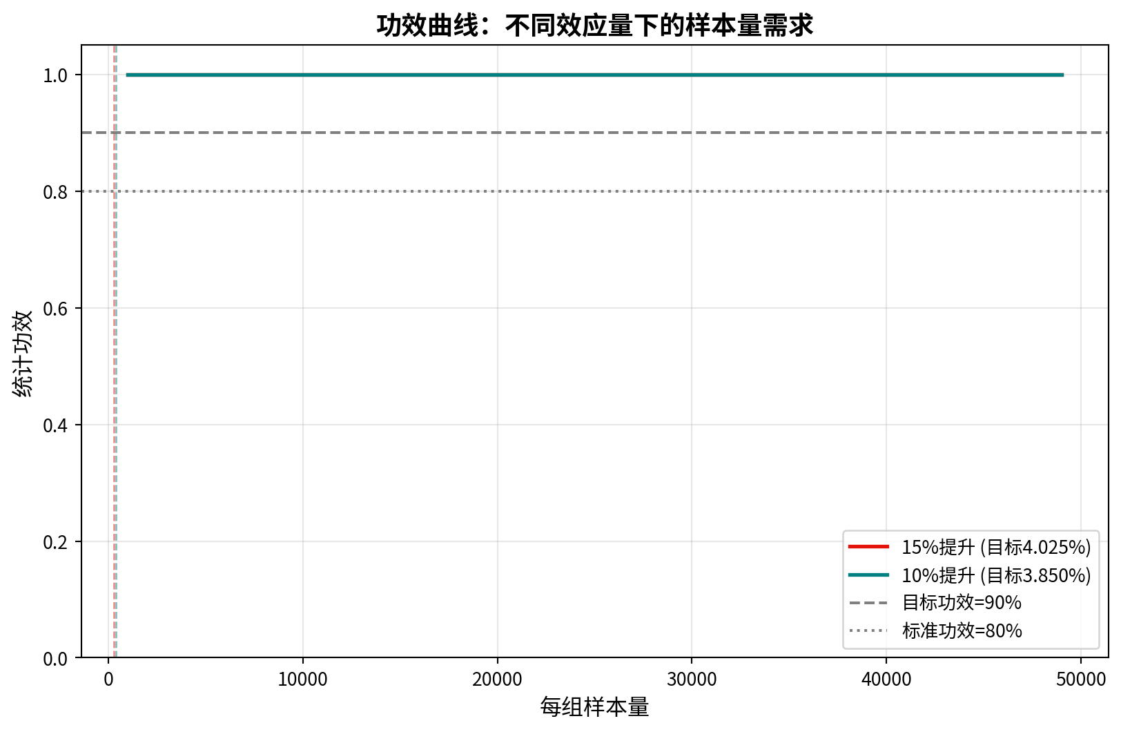
(3) 主要发现
  效应量越小(10% vs 15%),所需样本量越大
  样本量不足会导致功效降低,增加假阴性风险
  在设计A/B测试时,应基于最小可检测效应量计算样本量
上述功效曲线图直观展示了不同效应量下样本量与统计功效的关系。红色曲线(15%提升)和青色曲线(10%提升)均呈现典型的S形增长模式:随着每组样本量从1,000增加,功效迅速上升至接近1.0。垂直虚线标记了两种场景分别达到90%功效的最小样本量位置。三条关键发现总结了A/B测试设计的核心原则:(1)效应量越小,所需样本量越大,10%提升比15%提升多需约33%的样本;(2)样本量不足会降低功效,增加将有效策略误判为无效的假阴性风险;(3)在设计A/B测试时,应优先确定最小可检测效应量(MDE),再据此计算所需样本量,而非凭经验拍脑袋决定。
The power curve chart above intuitively illustrates the relationship between sample size and statistical power under different effect sizes. Both the red curve (15% lift) and the teal curve (10% lift) exhibit the typical S-shaped growth pattern: as the per-group sample size increases from 1,000, power rapidly rises toward 1.0. The vertical dashed lines mark the minimum sample size positions where each scenario achieves 90% power. Three key findings summarize the core principles of A/B test design: (1) smaller effect sizes require larger sample sizes — the 10% lift needs approximately 33% more samples than the 15% lift; (2) insufficient sample size reduces power and increases the risk of false negatives (incorrectly concluding an effective strategy is ineffective); (3) when designing A/B tests, one should first determine the minimum detectable effect (MDE) and then calculate the required sample size accordingly, rather than relying on arbitrary judgment.
习题 7.5 参考答案
Reference Solution to Exercise 7.5
# ========== 导入所需库 ==========
# ========== Import Required Libraries ==========
import numpy as np                                         # 导入numpy数值计算库
                                                           # Import numpy for numerical computation
import pandas as pd                                        # 导入pandas数据分析库
                                                           # Import pandas for data analysis
from scipy import stats                                    # 导入scipy统计检验模块
                                                           # Import scipy statistics module
import platform                                            # 导入平台检测模块
                                                           # Import platform detection module

# ========== 第1步:加载本地财务数据 ==========
# ========== Step 1: Load Local Financial Data ==========
if platform.system() == 'Windows':                         # 判断操作系统类型
                                                           # Determine operating system type
    data_path = 'C:/qiufei/data/stock'                     # Windows平台数据路径
                                                           # Data path for Windows platform
else:                                                      # 非Windows系统(Linux)
                                                           # Non-Windows system (Linux)
    data_path = '/home/ubuntu/r2_data_mount/qiufei/data/stock'  # Linux平台数据路径
                                                                  # Data path for Linux platform

stock_basic_info_dataframe = pd.read_hdf(f'{data_path}/stock_basic_data.h5')    # 读取上市公司基本信息
                                                                                          # Read listed company basic information
financial_statement_dataframe = pd.read_hdf(f'{data_path}/financial_statement.h5')  # 读取财务报表数据
                                                                                              # Read financial statement data

# ========== 第2步:筛选长三角地区上市公司 ==========
# ========== Step 2: Filter Yangtze River Delta Listed Companies ==========
yangtze_delta_provinces = ['上海市', '江苏省', '浙江省', '安徽省']  # 长三角四省市列表
                                                                     # List of four YRD provinces/municipalities
yrd_stock_codes_series = stock_basic_info_dataframe[  # 从基本信息中筛选长三角地区公司
                                                      # Filter YRD companies from basic information
    stock_basic_info_dataframe['province'].isin(yangtze_delta_provinces)  # 筛选长三角地区公司
                                                                          # Filter for YRD region companies
]['order_book_id']                                          # 提取股票代码
                                                           # Extract stock codes

# ========== 第3步:提取最新年报数据 ==========
# ========== Step 3: Extract Latest Annual Report Data ==========
financial_statement_dataframe = financial_statement_dataframe[  # 筛选年报数据
                                                                # Filter annual report data
    financial_statement_dataframe['quarter'].str.endswith('q4')  # 只保留第四季度(年报)数据
                                                                  # Keep only Q4 (annual report) data
]
financial_statement_dataframe = financial_statement_dataframe.sort_values('quarter', ascending=False)  # 按季度降序排列
                                                                                                       # Sort by quarter in descending order
financial_statement_dataframe = financial_statement_dataframe.drop_duplicates(  # 去重保留每家公司最新年报
                                                                                # Deduplicate to keep latest annual report per company
    subset='order_book_id', keep='first'                   # 每个公司只保留最新一期年报
                                                           # Keep only the most recent annual report for each company
)
长三角地区上市公司的最新年报数据提取完毕。下面筛选长三角公司、合并行业信息并计算ROE指标。
The latest annual report data for YRD listed companies has been extracted. Next, we filter for YRD companies, merge industry information, and compute the ROE indicator.
# ========== 第4步:筛选长三角公司并合并行业信息 ==========
# ========== Step 4: Filter YRD Companies and Merge Industry Information ==========
yrd_financial_dataframe = financial_statement_dataframe[  # 从财务数据中筛选长三角公司
                                                          # Filter YRD companies from financial data
    financial_statement_dataframe['order_book_id'].isin(yrd_stock_codes_series)  # 仅保留长三角公司
                                                                                 # Keep only YRD companies
].copy()                                                   # 创建副本避免链式赋值警告
                                                           # Create a copy to avoid chained assignment warning

yrd_financial_dataframe = yrd_financial_dataframe.merge(  # 合并行业信息和省份信息
                                                           # Merge industry and province information
    stock_basic_info_dataframe[['order_book_id', 'industry_name', 'province']],  # 合并行业名称和省份
                                                                                  # Merge industry name and province
    on='order_book_id', how='left'                         # 左连接,保留所有长三角公司
                                                           # Left join, keep all YRD companies
)

# ========== 第5步:计算ROE并去除异常值 ==========
# ========== Step 5: Compute ROE and Remove Outliers ==========
yrd_financial_dataframe['roe_percentage'] = (  # 计算净资产收益率ROE
                                                # Compute return on equity (ROE)
    yrd_financial_dataframe['net_profit'] / yrd_financial_dataframe['equity_parent_company']  # ROE = 净利润/归属母公司股东权益
                                                                                              # ROE = net profit / equity attributable to parent company
) * 100                                                    # 转换为百分比
                                                           # Convert to percentage

yrd_financial_dataframe = yrd_financial_dataframe[  # 去除ROE的缺失值和极端异常值
                                                     # Remove missing values and extreme outliers for ROE
    (yrd_financial_dataframe['roe_percentage'].notna()) &   # 去除缺失值
                                                            # Remove missing values
    (yrd_financial_dataframe['roe_percentage'] > -100) &    # 去除ROE<-100%的极端值
                                                            # Remove extreme values with ROE < -100%
    (yrd_financial_dataframe['roe_percentage'] < 100)       # 去除ROE>100%的极端值
                                                            # Remove extreme values with ROE > 100%
]
数据准备和ROE计算完成后,下面我们将长三角上市公司按行业类型分为制造业与非制造业两组,通过Welch’s t检验比较两组的ROE均值是否存在统计学意义上的显著差异,并计算效应量Hedges’ g和95%置信区间。
With data preparation and ROE computation complete, we now divide the YRD listed companies into two groups — manufacturing and non-manufacturing — by industry type, use Welch’s t-test to compare whether the mean ROE between the two groups differs significantly in a statistical sense, and calculate the effect size Hedges’ g along with the 95% confidence interval.
# ========== 第6步:定义制造业行业分类并分组 ==========
# ========== Step 6: Define Manufacturing Industry Classification and Group ==========
manufacturing_industries_list = [  # 定义制造业行业列表
                                    # Define list of manufacturing industries
    '计算机、通信和其他电子设备制造业', '汽车制造业', '专用设备制造业',         # 高端制造业
                                                                                # High-end manufacturing
    '电气机械和器材制造业', '化学原料和化学制品制造业',                        # 装备与化工制造业
                                                                                # Equipment and chemical manufacturing
    '医药制造业', '食品制造业', '纺织服装、服饰业', '造纸和纸制品业',          # 消费品制造业
                                                                                # Consumer goods manufacturing
    '非金属矿物制品业', '有色金属冶炼和压延加工业', '黑色金属冶炼和压延加工业'  # 原材料加工制造业
                                                                                  # Raw materials processing manufacturing
]

yrd_financial_dataframe['industry_type'] = yrd_financial_dataframe['industry_name'].apply(  # 新增行业类型分类列
                                                                                             # Add industry type classification column
    lambda x: '制造业' if x in manufacturing_industries_list else '非制造业'  # 按行业名称划分制造业与非制造业
                                                                              # Classify as manufacturing or non-manufacturing by industry name
)

manufacturing_roe_array = yrd_financial_dataframe[  # 提取制造业公司的ROE数据
                                                     # Extract ROE data for manufacturing companies
    yrd_financial_dataframe['industry_type'] == '制造业'    # 筛选制造业公司
                                                            # Filter manufacturing companies
]['roe_percentage'].values                                  # 提取ROE数组
                                                           # Extract ROE array
non_manufacturing_roe_array = yrd_financial_dataframe[  # 提取非制造业公司的ROE数据
                                                         # Extract ROE data for non-manufacturing companies
    yrd_financial_dataframe['industry_type'] == '非制造业'  # 筛选非制造业公司
                                                            # Filter non-manufacturing companies
]['roe_percentage'].values                                  # 提取ROE数组
                                                           # Extract ROE array
行业分组与ROE数组提取完毕。下面提出研究假设并输出描述性统计及方差齐性检验结果。
Industry grouping and ROE array extraction are complete. Next, we formulate the research hypothesis and output descriptive statistics and the variance homogeneity test results.
# ========== 第7步:提出研究假设 ==========
# ========== Step 7: Formulate Research Hypothesis ==========
print('=' * 60)                                          # 输出分隔线
                                                          # Print separator line
print('研究问题:长三角地区制造业与非制造业上市公司ROE是否存在差异?')  # 输出研究问题
                                                                         # Print research question
print('=' * 60)                                          # 输出分隔线
                                                          # Print separator line
print(f'H0: μ_制造业 - μ_非制造业 = 0')                     # 原假设:两组ROE无差异
                                                            # Null hypothesis: no difference in ROE between two groups
print(f'H1: μ_制造业 - μ_非制造业 ≠ 0')                     # 备择假设:两组ROE存在差异
                                                            # Alternative hypothesis: ROE differs between two groups

# ========== 第8步:输出探索性数据分析结果 ==========
# ========== Step 8: Output Exploratory Data Analysis Results ==========
print(f'\n描述性统计:')                                      # 描述性统计标题
                                                            # Descriptive statistics heading
print(f'制造业: n={len(manufacturing_roe_array)}, 均值={np.mean(manufacturing_roe_array):.2f}%, '  # 输出制造业描述性统计
                                                                                                     # Print manufacturing descriptive statistics
      f'标准差={np.std(manufacturing_roe_array, ddof=1):.2f}%')   # 制造业样本统计量
                                                                    # Manufacturing sample statistics
print(f'非制造业: n={len(non_manufacturing_roe_array)}, 均值={np.mean(non_manufacturing_roe_array):.2f}%, '  # 输出非制造业描述性统计
                                                                                                               # Print non-manufacturing descriptive statistics
      f'标准差={np.std(non_manufacturing_roe_array, ddof=1):.2f}%')  # 非制造业样本统计量
                                                                       # Non-manufacturing sample statistics

# ========== 第9步:Levene方差齐性检验 ==========
# ========== Step 9: Levene's Test for Equality of Variances ==========
from scipy.stats import levene                             # 导入Levene检验函数
                                                           # Import Levene test function
levene_stat, levene_p = levene(manufacturing_roe_array, non_manufacturing_roe_array)  # 执行Levene检验
                                                                                       # Perform Levene's test
print(f'\nLevene检验: W={levene_stat:.4f}, p={levene_p:.4f}')  # 输出Levene检验结果
                                                                  # Print Levene's test results
use_equal_var = levene_p > 0.05                            # 判断方差是否齐性(p>0.05则齐性)
                                                           # Determine variance homogeneity (homogeneous if p > 0.05)
============================================================
研究问题:长三角地区制造业与非制造业上市公司ROE是否存在差异?
============================================================
H0: μ_制造业 - μ_非制造业 = 0
H1: μ_制造业 - μ_非制造业 ≠ 0
描述性统计:
制造业: n=987, 均值=3.76%, 标准差=13.47%
非制造业: n=1015, 均值=3.23%, 标准差=15.86%
Levene检验: W=5.5820, p=0.0182上述描述性统计和方差齐性检验结果显示:长三角地区制造业上市公司共987家,平均ROE为3.76%,标准差为13.47%;非制造业上市公司共1,015家,平均ROE为3.23%,标准差为15.86%。Levene检验的W统计量为5.5820,p值为0.0182,小于0.05的显著性水平,因此拒绝方差齐性的原假设。两组的方差存在显著差异(非制造业的ROE离散程度更大),后续均值比较应采用不假设等方差的Welch’s t检验。
The descriptive statistics and variance homogeneity test results above show that there are 987 manufacturing listed companies in the YRD with a mean ROE of 3.76% and a standard deviation of 13.47%, and 1,015 non-manufacturing listed companies with a mean ROE of 3.23% and a standard deviation of 15.86%. The Levene test yields a W statistic of 5.5820 with a p-value of 0.0182, which is below the 0.05 significance level, so we reject the null hypothesis of equal variances. There is a significant difference in variances between the two groups (non-manufacturing ROE has greater dispersion), and the subsequent mean comparison should use Welch’s t-test, which does not assume equal variances.
方差齐性检验和描述性统计完成。下面执行Welch’s t检验并输出完整结果。
The variance homogeneity test and descriptive statistics are complete. Next, we perform Welch’s t-test and output the full results.
# ========== 第10步:执行Welch's t检验 ==========
# ========== Step 10: Perform Welch's t-Test ==========
welch_t_stat, welch_p_value = stats.ttest_ind(  # 执行Welch t检验(不假设方差齐性)
                                                  # Perform Welch t-test (not assuming equal variances)
    manufacturing_roe_array, non_manufacturing_roe_array, equal_var=False  # 使用Welch校正(不假设方差齐性)
                                                                           # Use Welch correction (not assuming equal variances)
)

# ========== 第11步:计算效应量和置信区间 ==========
# ========== Step 11: Compute Effect Size and Confidence Interval ==========
mean_diff = np.mean(manufacturing_roe_array) - np.mean(non_manufacturing_roe_array)  # 均值差(制造业-非制造业)
                                                                                      # Mean difference (manufacturing - non-manufacturing)
pooled_sd = np.sqrt(  # 计算合并标准差(用于效应量)
                       # Compute pooled standard deviation (for effect size)
    ((len(manufacturing_roe_array)-1)*np.var(manufacturing_roe_array, ddof=1) +   # 制造业组内方差加权
                                                                                    # Weighted within-group variance for manufacturing
     (len(non_manufacturing_roe_array)-1)*np.var(non_manufacturing_roe_array, ddof=1)) /  # 非制造业组内方差加权
                                                                                            # Weighted within-group variance for non-manufacturing
    (len(manufacturing_roe_array) + len(non_manufacturing_roe_array) - 2)          # 合并标准差(自由度权重)
                                                                                    # Pooled standard deviation (degrees of freedom weighting)
)
hedges_g = mean_diff / pooled_sd                           # 计算Hedges' g效应量
                                                           # Compute Hedges' g effect size

se_diff = np.sqrt(  # 计算均值差的标准误
                     # Compute standard error of the mean difference
    np.var(manufacturing_roe_array, ddof=1)/len(manufacturing_roe_array) +         # 制造业组标准误²
                                                                                    # Manufacturing group SE²
    np.var(non_manufacturing_roe_array, ddof=1)/len(non_manufacturing_roe_array)   # 非制造业组标准误²
                                                                                    # Non-manufacturing group SE²
)                                                          # 均值差的标准误
                                                           # Standard error of the mean difference
ci_lower = mean_diff - 1.96 * se_diff                     # 95%置信区间下界
                                                           # Lower bound of 95% confidence interval
ci_upper = mean_diff + 1.96 * se_diff                     # 95%置信区间上界
                                                           # Upper bound of 95% confidence interval
Welch t检验与效应量计算完毕。下面输出完整检验结果与研究结论。
Welch’s t-test and effect size computation are complete. Next, we output the full test results and research conclusions.
# ========== 第12步:输出检验结果 ==========
# ========== Step 12: Output Test Results ==========
print(f'\nWelch\'s t检验:')                                 # Welch t检验标题
                                                            # Welch's t-test heading
print(f'  t统计量: {welch_t_stat:.4f}')                     # t统计量
                                                            # t-statistic
print(f'  p值: {welch_p_value:.6f}')                        # p值
                                                            # p-value
print(f'  均值差: {mean_diff:.2f}%')                        # 均值差
                                                            # Mean difference
print(f'  95% CI: [{ci_lower:.2f}, {ci_upper:.2f}]%')      # 95%置信区间
                                                            # 95% confidence interval
print(f'  Hedges\' g: {hedges_g:.4f}')                      # Hedges' g效应量
                                                            # Hedges' g effect size

# ========== 第13步:输出研究结论 ==========
# ========== Step 13: Output Research Conclusions ==========
print(f'\n结论:')                                           # 结论标题
                                                            # Conclusion heading
if welch_p_value < 0.05:                                   # 显著性判断(α=0.05)
                                                            # Significance test (α = 0.05)
    print(f'  在α=0.05水平下拒绝H0,制造业与非制造业ROE存在显著差异')  # 拒绝原假设
                                                                         # Reject null hypothesis
else:                                                      # p值不显著的情形
                                                            # Case when p-value is not significant
    print(f'  在α=0.05水平下不能拒绝H0')                    # 不能拒绝原假设
                                                            # Fail to reject null hypothesis
print(f'数据来源: 本地financial_statement.h5 + stock_basic_data.h5')  # 标注数据来源
                                                                                 # Note data source
Welch's t检验:
  t统计量: 0.8058
  p值: 0.420434
  均值差: 0.53%
  95% CI: [-0.76, 1.82]%
  Hedges' g: 0.0359

结论:
  在α=0.05水平下不能拒绝H0
数据来源: 本地financial_statement.h5 + stock_basic_data.h5
上述Welch’s t检验结果显示:t统计量为0.8058,p值为0.420434,远大于α=0.05的显著性水平,因此不能拒绝原假设。制造业平均ROE(3.76%)仅比非制造业(3.23%)高0.53个百分点,均值差的95%置信区间为[-0.76, 1.82]%,包含0值。Hedges’ g效应量仅为0.0359,属于极小效应量(|g|<0.2),表明两组之间的实际差异几乎可以忽略不计。综上所述,在统计学意义和实际意义两个维度上,长三角地区制造业与非制造业上市公司的盈利能力(以ROE衡量)均不存在显著差异。该结论表明,就平均水平而言,行业类型并非决定长三角上市公司盈利能力的关键因素。
The Welch’s t-test results above show a t-statistic of 0.8058 and a p-value of 0.420434, far exceeding the α = 0.05 significance level, so we fail to reject the null hypothesis. The mean ROE for manufacturing (3.76%) is only 0.53 percentage points higher than for non-manufacturing (3.23%), and the 95% confidence interval for the mean difference is [−0.76, 1.82]%, which includes zero. The Hedges’ g effect size is only 0.0359, classified as a negligible effect (|g| < 0.2), indicating that the practical difference between the two groups is virtually negligible. In summary, on both statistical and practical significance dimensions, there is no significant difference in profitability (as measured by ROE) between manufacturing and non-manufacturing listed companies in the Yangtze River Delta region. This conclusion suggests that, on average, industry type is not a key determinant of profitability for YRD listed companies.
本章系统介绍了均值推断的三种核心方法——单样本t检验、两独立样本t检验和配对样本t检验——并结合中国A股上市公司的真实财务数据与股价数据进行了完整的实证演示。通过银行业净利润率检验、上海与广东股票收益率比较、银行股跨年收益率配对分析等案例,学生不仅掌握了假设检验的统计原理与Python实现,还深入理解了效应量、置信区间和统计功效等关键概念在商业决策中的实际意义。启发式思考部分通过噪声交易员模拟揭示了选择性偏差对t检验结论的影响,培养了学生对统计工具的批判性思维能力。
This chapter systematically introduced three core methods for inference about means — the one-sample t-test, the two-independent-samples t-test, and the paired-samples t-test — and provided complete empirical demonstrations using real financial and stock price data from Chinese A-share listed companies. Through cases such as the banking industry net profit margin test, the Shanghai versus Guangdong stock return comparison, and the paired analysis of bank stock returns across years, students not only mastered the statistical principles and Python implementation of hypothesis testing, but also gained a deep understanding of the practical significance of key concepts such as effect size, confidence intervals, and statistical power in business decision-making. The heuristic thinking section, through noise trader simulation, revealed the impact of selection bias on t-test conclusions, cultivating students’ critical thinking skills regarding statistical tools.