import pandas as pd          # 数据处理核心库
# Import the core data manipulation library
import numpy as np           # 数值计算核心库
# Import the core numerical computation library
from scipy.optimize import minimize  # 用于数值优化求解MLE
# Import the optimizer for numerically solving MLE
import matplotlib.pyplot as plt      # 数据可视化库
# Import the data visualization library
from pathlib import Path             # 跨平台路径处理
# Import cross-platform path handling utilities

# ---------- 中文字体配置 ----------
# ---------- Chinese Font Configuration ----------
plt.rcParams['font.sans-serif'] = ['SimHei']   # 设置中文字体为黑体,确保中文标签正常显示
# Set Chinese font to SimHei to ensure proper rendering of Chinese labels
plt.rcParams['axes.unicode_minus'] = False      # 关闭Unicode负号,避免负号显示为方块
# Disable Unicode minus sign to prevent display issues

# ========== 第1步:加载本地数据 ==========
# ========== Step 1: Load Local Data ==========
# 根据操作系统自动选择数据路径(Windows与Linux双平台兼容)
# Automatically select data path based on operating system (Windows/Linux compatible)
import platform  # 导入平台检测模块,用于判断当前操作系统
# Import platform detection module to determine the current OS
if platform.system() == 'Windows':  # 判断是否为Windows操作系统
    # Check if the current OS is Windows
    data_directory_path = Path('C:/qiufei/data/stock')    # Windows本地数据目录
    # Windows local data directory
else:  # 非Windows系统(Linux服务器环境)
    # Non-Windows system (Linux server environment)
    data_directory_path = Path('/home/ubuntu/r2_data_mount/qiufei/data/stock')  # Linux服务器数据目录
    # Linux server data directory

basic_info_file_path = data_directory_path / 'stock_basic_data.h5'        # 上市公司基本信息文件
# File path for listed company basic information
financial_statement_file_path = data_directory_path / 'financial_statement.h5'  # 财务报表文件
# File path for financial statements

# 读取HDF5格式数据,仅选取分析所需列以节省内存
# Read HDF5 data, selecting only the columns needed for analysis to save memory
basic_info_dataframe = pd.read_hdf(basic_info_file_path, columns=['order_book_id', 'province', 'industry_name'])  # 读取上市公司基本信息(代码、省份、行业)
# Read listed company basic info (stock code, province, industry)
financial_statement_dataframe = pd.read_hdf(financial_statement_file_path, columns=['order_book_id', 'quarter', 'net_profit', 'total_equity'])  # 读取财务报表(代码、季度、净利润、股东权益)
# Read financial statements (stock code, quarter, net profit, total equity)

# ========== 第2步:筛选长三角地区企业 ==========
# ========== Step 2: Filter YRD Region Companies ==========
yrd_provinces_list = ['上海市', '江苏省', '浙江省', '安徽省']  # 长三角四省市
# The four provinces/municipalities of the Yangtze River Delta
yrd_companies_dataframe = basic_info_dataframe[basic_info_dataframe['province'].isin(yrd_provinces_list)]  # 按省份筛选
# Filter by province5 推断统计基础 (Inferential Statistics)
推断统计是统计学的核心,它使我们能够从样本数据推断总体特征,并量化推断的不确定性。本章系统介绍点估计、区间估计和假设检验的理论与方法,这些方法是数据驱动决策的科学基础。
Inferential statistics is the core of statistics, enabling us to infer population characteristics from sample data and quantify the uncertainty of such inferences. This chapter systematically introduces the theory and methods of point estimation, interval estimation, and hypothesis testing—the scientific foundation of data-driven decision-making.
5.1 推断统计在金融市场研究中的典型应用 (Typical Applications of Inferential Statistics in Financial Market Research)
推断统计为金融市场的实证研究提供了严格的科学方法论。以下展示假设检验和区间估计在中国资本市场中的核心应用。
Inferential statistics provides a rigorous scientific methodology for empirical research in financial markets. The following demonstrates the core applications of hypothesis testing and interval estimation in China’s capital markets.
5.1.1 应用一:市场有效性的统计检验 (Application 1: Statistical Tests for Market Efficiency)
有效市场假说(EMH)认为,股票价格已充分反映所有可用信息,因此不存在持续获得超额收益的可能。检验这一假说的核心方法是假设检验:设立原假设 \(H_0\):市场有效(超额收益为零),备择假设 \(H_1\):存在可预测的超额收益。使用 stock_price_pre_adjusted.h5 中的历史收益率数据,可以对收益率的序列相关性进行检验。如果日收益率的一阶自相关显著不为零(即拒绝 \(H_0\)),则构成对弱式有效市场的证据反驳。
The Efficient Market Hypothesis (EMH) posits that stock prices fully reflect all available information, making it impossible to consistently earn excess returns. The core method for testing this hypothesis is hypothesis testing: set up the null hypothesis \(H_0\): the market is efficient (excess returns are zero), and the alternative hypothesis \(H_1\): predictable excess returns exist. Using historical return data from stock_price_pre_adjusted.h5, we can test the serial correlation of returns. If the first-order autocorrelation of daily returns is significantly different from zero (i.e., rejecting \(H_0\)), this constitutes evidence against weak-form market efficiency.
5.1.2 应用二:事件研究法中的异常收益检验 (Application 2: Abnormal Return Tests in Event Studies)
事件研究法(Event Study)通过检验事件窗口内的累积异常收益(CAR)是否显著异于零,来评估特定事件(如并购公告、政策变化、财报发布)对股价的影响。其统计基础是置信区间和t检验:如果CAR的95%置信区间不包含零,则认为该事件对股价有显著影响。基于 stock_price_pre_adjusted.h5 和 stock_basic_data.h5 中的实际数据,我们可以对长三角地区上市公司的重大事件进行实证分析。
The Event Study methodology assesses the impact of specific events (such as M&A announcements, policy changes, and earnings releases) on stock prices by testing whether the Cumulative Abnormal Return (CAR) within the event window is significantly different from zero. Its statistical foundation rests on confidence intervals and t-tests: if the 95% confidence interval for CAR does not contain zero, the event is considered to have a significant impact on stock prices. Based on actual data from stock_price_pre_adjusted.h5 and stock_basic_data.h5, we can conduct empirical analysis of major events for listed companies in the Yangtze River Delta region.
5.1.3 应用三:投资策略的统计显著性评估 (Application 3: Statistical Significance Assessment of Investment Strategies)
量化投资中,评估一个交易策略是否真正有效而非依靠”运气”,需要严格的假设检验。原假设为 \(H_0\):策略的真实超额收益为零(策略无效),通过统计检验量化策略表现的置信水平。结合 stock_price_pre_adjusted.h5 中的历史行情数据构建回测,并使用t检验评估策略收益的统计显著性,可以区分真正有效的Alpha策略和过拟合的”数据挖掘”结果。这体现了推断统计在投资实践中防范”p-hacking”和过度拟合的重要价值。
In quantitative investing, evaluating whether a trading strategy is genuinely effective rather than relying on “luck” requires rigorous hypothesis testing. The null hypothesis is \(H_0\): the strategy’s true excess return is zero (the strategy is ineffective), and statistical tests are used to quantify the confidence level of strategy performance. By constructing backtests using historical market data from stock_price_pre_adjusted.h5 and employing t-tests to assess the statistical significance of strategy returns, one can distinguish truly effective Alpha strategies from overfitted “data mining” results. This exemplifies the critical value of inferential statistics in guarding against “p-hacking” and overfitting in investment practice.
5.2 点估计 (Point Estimation)
5.2.1 估计量的性质 (Properties of Estimators)
5.2.1.1 无偏性 (Unbiasedness)
估计量 \(\hat{\theta}\) 是参数 \(\theta\) 的无偏估计,如果它满足 式 5.1 所示的条件:
An estimator \(\hat{\theta}\) is an unbiased estimator of the parameter \(\theta\) if it satisfies the condition shown in 式 5.1:
\[ E[\hat{\theta}] = \theta \tag{5.1}\]
常见无偏估计量:
- 样本均值 \(\bar{X}\) 是总体均值 \(\mu\) 的无偏估计
- 样本方差 \(S^2 = \frac{1}{n-1}\sum_{i=1}^n (X_i - \bar{X})^2\) 是总体方差 \(\sigma^2\) 的无偏估计
Common unbiased estimators:
- The sample mean \(\bar{X}\) is an unbiased estimator of the population mean \(\mu\)
- The sample variance \(S^2 = \frac{1}{n-1}\sum_{i=1}^n (X_i - \bar{X})^2\) is an unbiased estimator of the population variance \(\sigma^2\)
为什么样本方差用n-1?
Why does the sample variance use n-1?
回顾第2章的讨论:使用 \(n-1\) 而不是 \(n\) 是为了确保无偏性。
Recall the discussion in Chapter 2: using \(n-1\) instead of \(n\) is to ensure unbiasedness.
直观理解:当我们用样本均值 \(\bar{X}\) 代替总体均值 \(\mu\) 时,样本数据与 \(\bar{X}\) 的距离总是小于与真实 \(\mu\) 的距离。这会导致低估真实方差。除以 \(n-1\) 可以补偿这个偏差。
Intuitive understanding: when we substitute the sample mean \(\bar{X}\) for the population mean \(\mu\), the distances from the sample data to \(\bar{X}\) are always smaller than the distances to the true \(\mu\). This leads to an underestimation of the true variance. Dividing by \(n-1\) compensates for this bias.
5.2.1.2 有效性 (Efficiency)
在所有无偏估计量中,方差最小的估计量称为最有效估计量。
Among all unbiased estimators, the one with the smallest variance is called the most efficient estimator.
克拉默-拉奥下界(Cramér-Rao Lower Bound)给出了无偏估计量方差的理论下界。
The Cramér-Rao Lower Bound provides a theoretical lower bound for the variance of any unbiased estimator.
5.2.1.3 一致性 (Consistency)
估计量 \(\hat{\theta}_n\) (基于样本量 \(n\)) 是一致的,如果当 \(n \to \infty\) 时,它满足 式 5.2 所示的条件:
An estimator \(\hat{\theta}_n\) (based on sample size \(n\)) is consistent if, as \(n \to \infty\), it satisfies the condition shown in 式 5.2:
\[ \hat{\theta}_n \xrightarrow{p} \theta \tag{5.2}\]
即估计量依概率收敛于真实参数。
That is, the estimator converges in probability to the true parameter.
5.2.2 极大似然估计 (Maximum Likelihood Estimation, MLE)
直觉: 极大似然估计的核心思想非常朴素——“发生的事情是概率最大的”。如果在这个参数下,出现当前数据的概率最大,那么这个参数就是最”可信”的估计值。
Intuition: The core idea of maximum likelihood estimation is remarkably intuitive—“what happened is what was most likely to happen.” If the probability of observing the current data is maximized under a particular parameter value, then that parameter value is the most “credible” estimate.
数学推导: 以最简单的抛硬币(或企业盈亏)为例。设 \(X\) 服从伯努利分布 \(B(p)\),即 \(P(X=1)=p\) (盈利),\(P(X=0)=1-p\) (亏损)。 假设我们观察到 \(n\) 个独立样本 \(x_1, x_2, ..., x_n\)。
Mathematical Derivation: Consider the simplest example of a coin flip (or corporate profit/loss). Let \(X\) follow a Bernoulli distribution \(B(p)\), where \(P(X=1)=p\) (profitable) and \(P(X=0)=1-p\) (loss-making). Suppose we observe \(n\) independent samples \(x_1, x_2, ..., x_n\).
似然函数 (Likelihood Function) 是观测数据出现的联合概率,主要关于参数 \(p\) 的函数:
The Likelihood Function is the joint probability of the observed data as a function of the parameter \(p\):
\[ L(p) = P(x_1, ..., x_n | p) = \prod_{i=1}^n p^{x_i} (1-p)^{1-x_i} \] \[ L(p) = p^{\sum x_i} (1-p)^{n-\sum x_i} \]
为了计算方便,我们通常取对数(对数函数是单调递增的,最大化对数似然等价于最大化似然):
For computational convenience, we typically take the logarithm (since the logarithmic function is monotonically increasing, maximizing the log-likelihood is equivalent to maximizing the likelihood):
\[ \ell(p) = \ln L(p) = (\sum x_i) \ln p + (n-\sum x_i) \ln(1-p) \]
为了找到使 \(\ell(p)\) 最大的 \(p\),我们对 \(p\) 求导并令其为 0:
To find the value of \(p\) that maximizes \(\ell(p)\), we take the derivative with respect to \(p\) and set it equal to 0:
\[ \frac{d\ell}{dp} = \frac{\sum x_i}{p} - \frac{n-\sum x_i}{1-p} = 0 \]
解这个方程:
Solving this equation:
\[ (1-p)\sum x_i = p(n-\sum x_i) \] \[ \sum x_i - p\sum x_i = pn - p\sum x_i \] \[ p = \frac{\sum x_i}{n} = \bar{x} \]
结论:样本均值(即盈利公司的比例)就是总体比例 \(p\) 的极大似然估计量 \(\hat{p}_{MLE}\)。
Conclusion: The sample mean (i.e., the proportion of profitable companies) is the maximum likelihood estimator \(\hat{p}_{MLE}\) of the population proportion \(p\).
反例:MLE 总是最好的吗?
Counterexample: Is MLE Always the Best?
虽然 MLE 具有一致性(样本量很大时收敛到真值)和渐近正态性,但它并不总是无偏的。 一个经典的反例是方差的估计。对于正态分布 \(N(\mu, \sigma^2)\), \(\sigma^2\) 的 MLE 估计量是 \(\hat{\sigma}^2_{MLE} = \frac{1}{n}\sum(x_i - \bar{x})^2\)。 然而,这个估计量是有偏的(偏小)。为了纠正偏差,我们需要除以 \(n-1\)(即样本方差 \(S^2\))。这提醒我们:虽然 MLE 是寻找估计量的强力工具,但 blind application 可能会带来偏差,尤其是在小样本下。
Although MLE possesses consistency (converging to the true value as the sample size grows large) and asymptotic normality, it is not always unbiased. A classic counterexample is the estimation of variance. For a normal distribution \(N(\mu, \sigma^2)\), the MLE of \(\sigma^2\) is \(\hat{\sigma}^2_{MLE} = \frac{1}{n}\sum(x_i - \bar{x})^2\). However, this estimator is biased (biased downward). To correct for this bias, we need to divide by \(n-1\) (yielding the sample variance \(S^2\)). This reminds us that although MLE is a powerful tool for finding estimators, blind application can introduce bias, especially with small samples.
MLE的直观理解:客户满意度调查
Intuitive Understanding of MLE: Customer Satisfaction Survey
假设某公司想知道客户满意度 \(p\)。随机调查100人,85人表示满意。
Suppose a company wants to know its customer satisfaction rate \(p\). A random survey of 100 people reveals that 85 expressed satisfaction.
似然函数: \(L(p) = \binom{100}{85} p^{85} (1-p)^{15}\)
Likelihood function: \(L(p) = \binom{100}{85} p^{85} (1-p)^{15}\)
MLE: 求 \(L(p)\) 关于 \(p\) 的最大值,得到:
MLE: Maximizing \(L(p)\) with respect to \(p\), we obtain:
\[ \hat{p}_{MLE} = \frac{85}{100} = 0.85 \]
解释: 使”观察到85人满意”这个事件概率最大的 \(p\) 值就是0.85,即样本比例。这符合直觉。
Interpretation: The value of \(p\) that maximizes the probability of the event “85 out of 100 are satisfied” is 0.85, which is simply the sample proportion. This aligns with intuition.
5.2.2.1 案例:长三角上市公司盈利比例的极大似然估计 (Case Study: MLE of Profitability Ratio for YRD Listed Companies)
什么是企业盈利比例的估计?
What is the Estimation of Corporate Profitability Ratio?
在投资分析和信用评估中,了解某一区域或行业中「有多大比例的企业处于盈利状态」是一项基础且关键的指标。例如,银行在对长三角地区制造业企业进行批量授信时,需要评估该区域企业群体的整体盈利健康度。如果盈利比例过低,意味着该区域的信用风险较高,授信策略需要更加审慎。
In investment analysis and credit assessment, understanding “what proportion of companies in a given region or industry are profitable” is a fundamental and critical metric. For instance, when banks conduct batch credit approvals for manufacturing enterprises in the Yangtze River Delta region, they need to assess the overall profitability health of the corporate population in that area. If the profitability ratio is too low, it signals higher credit risk in the region, necessitating more prudent lending strategies.
极大似然估计(MLE)是估计此类「总体比例」参数的经典统计方法。其核心思想是:在所有可能的参数值中,找到那个使我们「实际观察到的样本数据出现概率最大」的参数值。下面我们使用本地上市公司财务数据,通过极大似然估计法计算长三角地区上市公司的盈利比例,结果如 表 5.1 所示。
Maximum Likelihood Estimation (MLE) is the classic statistical method for estimating such “population proportion” parameters. Its core idea is: among all possible parameter values, find the one that maximizes the probability of the sample data we actually observed. Below, we use local listed company financial data to compute the profitability ratio of YRD listed companies via MLE, with results shown in 表 5.1.
长三角地区上市公司基本信息筛选完毕。下面合并目标季度的财务数据并计算盈利状态。
The basic information of YRD listed companies has been filtered. Next, we merge the target quarter’s financial data and compute profitability status.
# ========== 第3步:获取目标季度财务数据 ==========
# ========== Step 3: Retrieve Target Quarter Financial Data ==========
# 选取2023年第3季度数据作为分析样本
# Select Q3 2023 data as the analysis sample
target_quarter_string = '2023q3'  # 目标分析季度:2023年第三季度
# Target analysis quarter: Q3 2023
financial_statement_quarter_dataframe = financial_statement_dataframe[  # 从财务报表中筛选指定季度
    financial_statement_dataframe['quarter'] == target_quarter_string  # 筛选目标季度
]
# Filter the target quarter from financial statements

# 将公司基本信息与财务数据按股票代码(order_book_id)内连接合并
# Inner join company basic info with financial data on stock code (order_book_id)
merged_analysis_dataframe = pd.merge(yrd_companies_dataframe, financial_statement_quarter_dataframe, on='order_book_id', how='inner')  # 内连接保留双表匹配记录
# Inner join retains only records matching in both tables

# 定义盈利状态:净利润大于0标记为1(盈利),否则为0(亏损)
# Define profitability status: net profit > 0 marked as 1 (profitable), otherwise 0 (loss-making)
merged_analysis_dataframe['is_profitable'] = (merged_analysis_dataframe['net_profit'] > 0).astype(int)  # 盈利标志:1=盈利,0=亏损
# Profitability flag: 1 = profitable, 0 = loss-making

# 统计样本总数和盈利企业数
# Count total sample size and number of profitable companies
total_companies_count = len(merged_analysis_dataframe)          # 总样本量n
# Total sample size n
profitable_companies_count = merged_analysis_dataframe['is_profitable'].sum()  # 盈利企业数k
# Number of profitable companies k
长三角地区上市公司盈利数据准备完成。下面通过极大似然估计法求解盈利比例的点估计。
The profitability data for YRD listed companies is now prepared. Next, we solve for the point estimate of the profitability ratio using maximum likelihood estimation.
# ========== 第4步:极大似然估计 ==========
# ========== Step 4: Maximum Likelihood Estimation ==========
# 定义负对数似然函数(因为scipy.optimize.minimize执行最小化,所以取负号)
# Define the negative log-likelihood function (negated because scipy.optimize.minimize performs minimization)
def calculate_negative_log_likelihood(probability_parameter):  # 接收候选概率参数p
    # Takes a candidate probability parameter p
    # 将参数p裁剪到(0,1)开区间内,避免log(0)导致数值错误
    # Clip parameter p to the open interval (0,1) to avoid numerical errors from log(0)
    probability_parameter = np.clip(probability_parameter, 1e-10, 1-1e-10)  # 数值稳定性处理:限制p在极小正数到接近1之间
    # Numerical stability: constrain p between a tiny positive number and near 1
    # 二项分布对数似然: log L(p) = k*log(p) + (n-k)*log(1-p) + 常数项
    # Binomial log-likelihood: log L(p) = k*log(p) + (n-k)*log(1-p) + constant term
    # 这里忽略组合数常数项(它不影响最优解的位置)
    # The combinatorial constant is omitted here (it does not affect the location of the optimum)
    return -(profitable_companies_count * np.log(probability_parameter) +  # 负对数似然:k*log(p)
    # Negative log-likelihood: k*log(p)
             (total_companies_count - profitable_companies_count) * np.log(1-probability_parameter))  # 加上(n-k)*log(1-p)
    # Plus (n-k)*log(1-p)

# 使用L-BFGS-B算法在[0.001, 0.999]范围内数值求解最大似然估计
# Use the L-BFGS-B algorithm to numerically solve the MLE within the [0.001, 0.999] range
optimization_result = minimize(calculate_negative_log_likelihood, x0=0.5, bounds=[(0.001, 0.999)])  # 初始值0.5,约束p∈[0.001,0.999]
# Initial value 0.5, constraint p ∈ [0.001, 0.999]
mle_estimated_probability = optimization_result.x[0]          # 数值优化得到的MLE估计值
# MLE estimate obtained via numerical optimization
theoretical_probability = profitable_companies_count / total_companies_count  # 理论公式: p_hat = k/n
# Theoretical formula: p_hat = k/n
基于上述数据准备和MLE参数估计,我们输出估计结果并绘制似然函数曲线,直观展示极大似然估计的原理:
Based on the data preparation and MLE parameter estimation above, we output the estimation results and plot the likelihood function curve to visually demonstrate the principle of maximum likelihood estimation:
# ========== 第5步:输出结果 ==========
# ========== Step 5: Output Results ==========
print(f'数据来源: 本地数据集 (长三角地区上市公司 {target_quarter_string} 财报)')  # 标注数据来源
# Print data source annotation
print(f'样本总数: {total_companies_count} 家')  # 输出总样本量
# Print total sample size
print(f'盈利家数: {profitable_companies_count} 家')  # 输出盈利企业数
# Print number of profitable companies
print(f'MLE估计 (数值优化): {mle_estimated_probability:.6f}')     # 数值解
# MLE estimate (numerical optimization)
print(f'MLE估计 (理论公式): {theoretical_probability:.6f}')       # 解析解(两者应一致)
# MLE estimate (theoretical formula) — both should be identical
print(f'盈利比例: {theoretical_probability:.2%}')  # 以百分比格式输出盈利比例
# Print profitability ratio in percentage format
数据来源: 本地数据集 (长三角地区上市公司 2023q3 财报)
样本总数: 1978 家
盈利家数: 1678 家
MLE估计 (数值优化): 0.848332
MLE估计 (理论公式): 0.848332
盈利比例: 84.83%表 5.1 的输出结果揭示了长三角上市公司的盈利全景:在2023年第三季度,1978家样本企业中有1678家实现盈利,MLE估计的盈利比例为 \(\hat{p} = 0.8483\)(约84.83%)。值得注意的是,数值优化法(SciPy的minimize)和理论公式法(\(\hat{p} = k/n\))给出了完全一致的结果(0.848332),这验证了我们在理论推导中证明的结论——对于伯努利试验,MLE的解析解与数值解相同。从经济含义来看,约85%的盈利比例表明长三角制造业上市公司整体盈利健康度较高,但仍有约15%的企业处于亏损状态,这对银行批量授信的风控策略具有重要参考价值。
The output of 表 5.1 reveals the full profitability picture of YRD listed companies: in Q3 2023, out of 1,978 sample firms, 1,678 were profitable, with the MLE-estimated profitability ratio of \(\hat{p} = 0.8483\) (approximately 84.83%). Notably, the numerical optimization method (SciPy’s minimize) and the theoretical formula (\(\hat{p} = k/n\)) yield identical results (0.848332), verifying the conclusion proven in our theoretical derivation—for Bernoulli trials, the analytical and numerical solutions of MLE are the same. From an economic perspective, a profitability ratio of approximately 85% indicates that YRD manufacturing listed companies are in generally healthy profitability condition, yet about 15% remain in a loss-making state, which carries important implications for banks’ risk management strategies in batch credit approvals.
下面绘制似然函数曲线,直观展示MLE的原理。
Below, we plot the likelihood function curve to visually illustrate the principle of MLE.
# ========== 第6步:可视化似然函数 ==========
# ========== Step 6: Visualize the Likelihood Function ==========
# 在[0.5, 1.0]区间内构建100个候选概率值(盈利比例通常较高)
# Construct 100 candidate probability values in the [0.5, 1.0] interval (profitability ratios are typically high)
probability_values_array = np.linspace(0.5, 1.0, 100)  # 生成100个等距候选概率值
# Generate 100 equally spaced candidate probability values
# 计算每个候选概率值对应的似然值(取指数还原为似然而非对数似然)
# Compute the likelihood value for each candidate (exponentiate to recover likelihood from log-likelihood)
likelihood_values_list = [np.exp(-calculate_negative_log_likelihood(p)) for p in probability_values_array]  # 对每个p计算似然值L(p)
# Compute likelihood L(p) for each candidate p
# 归一化处理:将最大似然值缩放为1,便于绘图比较
# Normalization: scale the maximum likelihood value to 1 for easier visual comparison
normalized_likelihood_values_array = np.array(likelihood_values_list) / np.max(likelihood_values_list)  # 归一化:最大值=1
# Normalize: maximum value = 1

# 绘制归一化似然函数曲线
# Plot the normalized likelihood function curve
mle_figure, mle_axes = plt.subplots(figsize=(10, 6))  # 创建10×6英寸画布与坐标轴对象
# Create a 10×6 inch figure and axes object
mle_axes.plot(probability_values_array, normalized_likelihood_values_array, 'b-', linewidth=2.5, label='归一化似然函数')  # 绘制蓝色实线似然曲线
# Plot the blue solid likelihood curve
# 用红色虚线标注MLE估计值的位置(似然函数的峰值点)
# Mark the MLE estimate position with a red dashed line (the peak of the likelihood function)
mle_axes.axvline(mle_estimated_probability, color='red', linestyle='--', linewidth=2, label=f'MLE = {mle_estimated_probability:.4f}')  # 红色虚线标注MLE估计值位置
# Red dashed line marking the MLE estimate position

mle_axes.set_xlabel('盈利比例 (p)', fontsize=12)       # X轴:候选参数值
# X-axis: candidate parameter values
mle_axes.set_ylabel('相对似然值', fontsize=12)          # Y轴:归一化似然值
# Y-axis: normalized likelihood values
mle_axes.set_title(f'长三角上市公司盈利比例的MLE估计 ({target_quarter_string})', fontsize=14)  # 设置图表标题
# Set the chart title
mle_axes.legend(fontsize=11)                             # 显示图例
# Display the legend
mle_axes.grid(True, alpha=0.3)                           # 添加半透明网格线
# Add semi-transparent grid lines

plt.tight_layout()  # 自动调整子图间距,防止标签被截断
# Automatically adjust subplot spacing to prevent label clipping
plt.show()           # 渲染并显示图形
# Render and display the figure
图 5.1 直观展示了似然函数的核心原理。曲线呈现明显的单峰钟形结构,在 \(p \approx 0.848\) 处达到最大值(归一化似然值为1.0),这正是MLE估计值的位置,由红色虚线标注。曲线的尖锐程度反映了估计的精度——由于样本量较大(\(n = 1978\)),似然函数在峰值附近急剧下降,表明MLE估计的不确定性很小。直观地说,如果曲线在峰值两侧缓慢下降,意味着多个候选参数值的似然函数值都接近最大值,估计就不够精确;而本案例中曲线陡峭的衰减,说明数据强烈”偏好”\(\hat{p} = 0.848\) 这一估计值,其他候选值的可能性迅速降低。
图 5.1 visually demonstrates the core principle of the likelihood function. The curve exhibits a clear unimodal bell-shaped structure, reaching its maximum (normalized likelihood value of 1.0) at \(p \approx 0.848\), which is precisely the location of the MLE estimate, marked by the red dashed line. The sharpness of the curve reflects the precision of the estimate—because the sample size is large (\(n = 1978\)), the likelihood function drops steeply near the peak, indicating very low uncertainty in the MLE estimate. Intuitively, if the curve declined slowly on both sides of the peak, it would mean that multiple candidate parameter values have likelihood values close to the maximum, resulting in an imprecise estimate. In this case, however, the steep decay of the curve indicates that the data strongly “favors” the estimate \(\hat{p} = 0.848\), with the plausibility of other candidate values diminishing rapidly. ## 区间估计 (Interval Estimation) {#sec-interval-estimation}
5.2.3 置信区间的概念与几何解释 (Concept and Geometric Interpretation of Confidence Intervals)
直觉: 点估计(如平均 ROE 为 8.5%)就像是用一支箭去射靶心,虽然瞄得很准,但射中靶心(精确等于真值)的概率几乎为0。 置信区间就像是撒一张网。我们无法保证网的中心就在靶心,但我们可以保证这张网的大小足以在 95% 的投掷中”网住”靶心。
Intuition: A point estimate (e.g., an average ROE of 8.5%) is like shooting a single arrow at a bullseye — although well-aimed, the probability of hitting the exact center (equaling the true value precisely) is virtually zero. A confidence interval is like casting a net. We cannot guarantee that the center of the net lies on the bullseye, but we can ensure the net is large enough to “capture” the bullseye in 95% of the throws.
数学推导 (Normal Case): 假设样本均值 \(\bar{X} \sim N(\mu, \sigma^2/n)\)。如果不确定性标准化,我们得到枢轴量 (Pivotal Quantity) \(Z\): \[ Z = \frac{\bar{X} - \mu}{\sigma/\sqrt{n}} \sim N(0, 1) \]
Mathematical Derivation (Normal Case): Assume the sample mean \(\bar{X} \sim N(\mu, \sigma^2/n)\). If we standardize the uncertainty, we obtain the pivotal quantity \(Z\): \[ Z = \frac{\bar{X} - \mu}{\sigma/\sqrt{n}} \sim N(0, 1) \]
我们知道标准正态分布有 95% 的概率落在 \([-1.96, 1.96]\) 之间: \[ P\left(-1.96 \le \frac{\bar{X} - \mu}{\sigma/\sqrt{n}} \le 1.96\right) = 0.95 \]
We know that the standard normal distribution has a 95% probability of falling within \([-1.96, 1.96]\): \[ P\left(-1.96 \le \frac{\bar{X} - \mu}{\sigma/\sqrt{n}} \le 1.96\right) = 0.95 \]
现在,我们通过代数变换,将 \(\mu\) 留在不等式中间: \[ P\left(\bar{X} - 1.96\frac{\sigma}{\sqrt{n}} \le \mu \le \bar{X} + 1.96\frac{\sigma}{\sqrt{n}}\right) = 0.95 \]
Now, through algebraic manipulation, we isolate \(\mu\) in the middle of the inequality: \[ P\left(\bar{X} - 1.96\frac{\sigma}{\sqrt{n}} \le \mu \le \bar{X} + 1.96\frac{\sigma}{\sqrt{n}}\right) = 0.95 \]
这就构成了 95% 的置信区间:\([\bar{X} - 1.96 SE, \bar{X} + 1.96 SE]\)。
This constitutes the 95% confidence interval: \([\bar{X} - 1.96 SE, \bar{X} + 1.96 SE]\).
概念陷阱:置信区间的解释
Conceptual Pitfall: Interpreting Confidence Intervals
❌ 错误:“也就是说明总体均值 \(\mu\) 有 95% 的概率落在这个区间内。” ✅ 正确:“该区间构建方法(Method)在长期重复使用中,有 95% 的区间会覆盖真实的 \(\mu\)。”
❌ Incorrect: “This means the population mean \(\mu\) has a 95% probability of falling within this interval.” ✅ Correct: “This interval construction method, when used repeatedly over the long run, will produce intervals that cover the true \(\mu\) 95% of the time.”
解释:在频率学派框架下,参数 \(\mu\) 是一个固定的常数,它要么在区间里,要么不在(概率为 1 或 0)。随机的是区间本身(因为样本 \(\bar{X}\) 是随机的)。
Explanation: Under the frequentist framework, the parameter \(\mu\) is a fixed constant — it is either inside the interval or not (with probability 1 or 0). What is random is the interval itself (because the sample mean \(\bar{X}\) is random).
想象你扔圈圈套娃娃。娃娃(\(\mu\))不动,你的圈圈(区间)是随机落下的。95% 置信水平衡量的是你扔圈圈的技术(方法的可靠性),而不是某个特定圈圈套中娃娃的概率。
Imagine tossing rings at a doll. The doll (\(\mu\)) stays put while your ring (the interval) lands randomly. The 95% confidence level measures your ring-tossing skill (the reliability of the method), not the probability that any particular ring has caught the doll.
5.2.4 均值的置信区间 (Confidence Interval for the Mean)
5.2.4.1 已知 \(\sigma\) 时 (When \(\sigma\) Is Known)
\(\mu\) 的 \(100(1-\alpha)\%\) 置信区间如 式 5.3 所示:
The \(100(1-\alpha)\%\) confidence interval for \(\mu\) is given by 式 5.3:
\[ \bar{X} \pm z_{\alpha/2} \frac{\sigma}{\sqrt{n}} \tag{5.3}\]
其中 \(z_{\alpha/2}\) 是标准正态分布的 \(\alpha/2\) 上侧分位数。
where \(z_{\alpha/2}\) is the upper \(\alpha/2\) quantile of the standard normal distribution.
5.2.4.2 未知 \(\sigma\) 时 (When \(\sigma\) Is Unknown)
使用样本标准差 \(S\) 替代 \(\sigma\),置信区间如 式 5.4 所示:
When the sample standard deviation \(S\) is used in place of \(\sigma\), the confidence interval is given by 式 5.4:
\[ \bar{X} \pm t_{\alpha/2, n-1} \frac{S}{\sqrt{n}} \tag{5.4}\]
其中 \(t_{\alpha/2, n-1}\) 是自由度为 \(n-1\) 的t分布的 \(\alpha/2\) 上侧分位数。
where \(t_{\alpha/2, n-1}\) is the upper \(\alpha/2\) quantile of the \(t\)-distribution with \(n-1\) degrees of freedom.
5.2.4.3 案例:平均消费支出估计 (Case Study: Estimating Average ROE)
什么是ROE的区间估计?
What Is an Interval Estimate of ROE?
净资产收益率(ROE)是衡量企业利用股东权益创造利润能力的核心指标,被巴菲特等价值投资者视为最重要的财务指标之一。当我们想了解「长三角电子行业上市公司的平均盈利能力如何」时,仅依靠一个样本均值(点估计)是不够的,因为它无法告诉我们这个估计值的精确度。
Return on Equity (ROE) is a core metric measuring a firm’s ability to generate profit from shareholders’ equity, regarded by value investors such as Warren Buffett as one of the most important financial indicators. When we ask “what is the average profitability of listed electronics companies in the Yangtze River Delta?”, relying on a single sample mean (point estimate) is insufficient, because it tells us nothing about the precision of that estimate.
置信区间为我们提供了一个「可信的范围」:它不仅给出平均ROE的估计值,还告诉我们在给定置信水平下,真实的总体均值最可能落在什么范围内。这对于行业对标分析和投资决策具有重要的实际意义。下面我们使用本地财务数据,构建长三角电子行业上市公司平均ROE的置信区间,结果如 表 5.2 所示。
A confidence interval provides a “credible range”: it not only gives the estimated average ROE but also tells us, at a given confidence level, within what range the true population mean is most likely to fall. This is of great practical significance for industry benchmarking and investment decisions. Below, we use local financial data to construct a confidence interval for the average ROE of listed electronics companies in the Yangtze River Delta, with results shown in 表 5.2.
import numpy as np  # 导入数值计算库
# Import the numerical computation library
import pandas as pd  # 导入数据处理库
# Import the data processing library
from scipy import stats  # 导入统计分布与检验模块
# Import the statistical distributions and hypothesis testing module
from pathlib import Path  # 导入路径处理模块,跨平台兼容
# Import the path handling module for cross-platform compatibility

# ---------- 加载本地数据 ----------
# ---------- Load local data ----------
import platform  # 导入平台检测模块,用于判断操作系统
# Import the platform detection module to identify the operating system
if platform.system() == 'Windows':  # Windows系统使用本地路径
    # Use the local path for Windows systems
    data_directory_path = Path('C:/qiufei/data/stock')  # Windows本地数据路径
    # Windows local data path
else:  # Linux服务器环境
    # Linux server environment
    data_directory_path = Path('/home/ubuntu/r2_data_mount/qiufei/data/stock')  # Linux本地数据路径
    # Linux local data path
basic_info_dataframe = pd.read_hdf(data_directory_path / 'stock_basic_data.h5')       # 加载公司基本信息
# Load company basic information
financial_statement_dataframe = pd.read_hdf(data_directory_path / 'financial_statement.h5')  # 加载财务报表
# Load financial statements

# ========== 第1步:数据准备——筛选长三角电子行业企业 ==========
# ========== Step 1: Data preparation — filter YRD electronics companies ==========
yrd_provinces_list = ['上海市', '江苏省', '浙江省', '安徽省']              # 长三角四省市
# The four YRD provinces/municipalities
target_industry_name = '计算机、通信和其他电子设备制造业'                  # 国统局行业分类代码对应的电子行业
# NBS industry classification code for the electronics sector
target_quarter_string = '2023q3'                                           # 分析的目标季度
# Target quarter for analysis

# 构建布尔掩码进行精确筛选(本地数据使用国统局行业分类标准)
# Construct boolean masks for precise filtering (local data uses NBS industry classification)
region_mask = basic_info_dataframe['province'].isin(yrd_provinces_list)     # 地区筛选:省份在长三角列表中
# Region filter: province is in the YRD list
industry_mask = basic_info_dataframe['industry_name'] == target_industry_name  # 行业筛选:精确匹配行业名称
# Industry filter: exact match of industry name
target_companies_dataframe = basic_info_dataframe[region_mask & industry_mask]  # 取交集:同时满足地区和行业条件
# Intersection: companies satisfying both region and industry conditions
长三角电子行业目标企业筛选完毕。下面获取目标季度财务数据,合并后计算ROE并清洗异常值。
Filtering of target YRD electronics companies is complete. Next, we retrieve financial data for the target quarter, merge the datasets, compute ROE, and clean outliers.
# 获取目标季度的财务报表数据
# Retrieve financial statement data for the target quarter
financial_statement_quarter_dataframe = financial_statement_dataframe[  # 筛选指定季度财务数据
    # Filter financial data for the specified quarter
    financial_statement_dataframe['quarter'] == target_quarter_string  # 筛选目标季度
    # Select the target quarter
].copy()  # 使用copy()避免SettingWithCopyWarning
# Use copy() to avoid SettingWithCopyWarning

# 将公司信息与财务数据内连接合并(只保留同时有基本信息和财务数据的公司)
# Inner-join company information with financial data (keep only companies with both)
merged_analysis_dataframe = pd.merge(target_companies_dataframe, financial_statement_quarter_dataframe, on='order_book_id', how='inner')  # 按股票代码内连接合并
# Inner join on stock code

# ========== 第2步:计算ROE(净资产收益率) ==========
# ========== Step 2: Compute ROE (Return on Equity) ==========
# ROE = 净利润 / 股东权益,衡量公司利用股东投入资本的获利效率
# ROE = Net Profit / Total Equity, measuring a firm's efficiency in generating profit from shareholders' capital
merged_analysis_dataframe['roe'] = merged_analysis_dataframe['net_profit'] / merged_analysis_dataframe['total_equity']  # 计算净资产收益率
# Compute Return on Equity

# ========== 第3步:数据清洗——处理异常值 ==========
# ========== Step 3: Data cleaning — handle outliers ==========
# 将无穷大值替换为NaN,并删除ROE为缺失值的行(分母为0时会产生inf)
# Replace infinity with NaN and drop rows where ROE is missing (inf arises when the denominator is zero)
merged_analysis_dataframe = merged_analysis_dataframe.replace([np.inf, -np.inf], np.nan).dropna(subset=['roe'])  # 清洗异常值
# Clean outliers
# 去除极端离群值:仅保留ROE在(-50%, 50%)范围内的观测(壳股或ST公司的ROE可能极端异常)
# Remove extreme outliers: keep only observations with ROE in (-50%, 50%) (shell companies or ST firms may have extreme ROE)
clean_analysis_dataframe = merged_analysis_dataframe[  # 筛选ROE合理范围内的样本
    # Filter samples within a reasonable ROE range
    (merged_analysis_dataframe['roe'] > -0.5) & (merged_analysis_dataframe['roe'] < 0.5)  # ROE取值范围约束
    # ROE range constraint
]

roe_sample_series = clean_analysis_dataframe['roe']  # 提取清洗后的ROE序列
# Extract the cleaned ROE series
sample_size_n = len(roe_sample_series)                # 有效样本量
# Effective sample size
完成数据筛选和清洗后,我们基于清洁样本计算描述性统计量,并构建不同置信水平下的区间估计:
After completing data filtering and cleaning, we compute descriptive statistics from the clean sample and construct interval estimates at different confidence levels:
# ========== 第4步:计算描述性统计量 ==========
# ========== Step 4: Compute descriptive statistics ==========
sample_mean_roe = roe_sample_series.mean()                          # 样本均值:ROE的点估计
# Sample mean: point estimate of ROE
sample_standard_deviation = roe_sample_series.std()                 # 样本标准差:衡量ROE的离散程度
# Sample standard deviation: measures the dispersion of ROE
standard_error = sample_standard_deviation / np.sqrt(sample_size_n) # 标准误:均值估计的不确定性
# Standard error: uncertainty of the mean estimate

# ========== 第5步:构建不同置信水平的置信区间 ==========
# ========== Step 5: Construct confidence intervals at different confidence levels ==========
confidence_levels_list = [0.90, 0.95, 0.99]  # 三个常用置信水平
# Three commonly used confidence levels
confidence_interval_results_list = []         # 存储结果的列表
# List to store results

for current_confidence_level in confidence_levels_list:  # 遍历三个置信水平
    # Iterate over the three confidence levels
    significance_level_alpha = 1 - current_confidence_level                          # 显著性水平α
    # Significance level α
    t_critical_value = stats.t.ppf(1 - significance_level_alpha/2, df=sample_size_n-1)  # t分布临界值(自由度=n-1)
    # t-distribution critical value (degrees of freedom = n-1)
    margin_of_error = t_critical_value * standard_error                              # 边际误差 = t临界值 × 标准误
    # Margin of error = t critical value × standard error

    confidence_interval_lower_bound = sample_mean_roe - margin_of_error  # 置信区间下界
    # Lower bound of the confidence interval
    confidence_interval_upper_bound = sample_mean_roe + margin_of_error  # 置信区间上界
    # Upper bound of the confidence interval

    # 将当前置信水平的结果存入字典
    # Store the results for the current confidence level in a dictionary
    confidence_interval_results_list.append({  # 将当前置信水平的结果存入字典
        # Append the current confidence level results to the list
        '置信水平': f'{current_confidence_level:.0%}',  # 格式化为百分比
        # Format as percentage
        't临界值': f'{t_critical_value:.3f}',  # t分布临界值
        # t-distribution critical value
        '标准误': f'{standard_error:.4f}',  # 均值估计的标准误
        # Standard error of the mean estimate
        '边际误差': f'{margin_of_error:.4f}',  # 置信区间的半宽
        # Half-width of the confidence interval
        '置信区间': f'[{confidence_interval_lower_bound:.2%}, {confidence_interval_upper_bound:.2%}]',  # 区间范围
        # Interval range
        '区间宽度': f'{confidence_interval_upper_bound - confidence_interval_lower_bound:.2%}'  # 区间总宽度
        # Total width of the interval
    })

# 将结果列表转换为DataFrame,方便展示
# Convert the result list to a DataFrame for display
results_summary_dataframe = pd.DataFrame(confidence_interval_results_list)  # 构建置信区间对比表
# Build the confidence interval comparison table
三种置信水平的区间计算完成。下面整理并输出置信区间对比表及经济学解释。
The interval calculations for all three confidence levels are complete. Below we compile and output the confidence interval comparison table along with the economic interpretation.
# ========== 第6步:输出分析结论 ==========
# ========== Step 6: Output the analytical conclusions ==========
print(f'分析对象: 长三角地区 {target_industry_name} 行业上市公司 ({target_quarter_string})')  # 打印分析范围
# Print the scope of the analysis
print(f'有效样本量: {sample_size_n} 家')  # 打印有效样本量
# Print the effective sample size
print(f'样本平均ROE: {sample_mean_roe:.2%}')                # 点估计结果
# Point estimate result
print(f'样本标准差: {sample_standard_deviation:.2%}')        # 离散程度
# Degree of dispersion
print(f'\n不同置信水平的区间估计:')  # 分隔标题
# Section heading
print(results_summary_dataframe)                              # 三个置信水平的对比表
# Comparison table for the three confidence levels

# 对95%置信区间的经济学解释
# Economic interpretation of the 95% confidence interval
print(f'\n解释:')  # 经济学解释部分
# Interpretation section
print(f'我们有95%的把握认为,长三角电子行业上市公司的平均ROE落在 [{sample_mean_roe - stats.t.ppf(0.975, sample_size_n-1)*standard_error:.2%}, {sample_mean_roe + stats.t.ppf(0.975, sample_size_n-1)*standard_error:.2%}] 之间。')  # 输出95%置信区间的业务含义
# Output the business implication of the 95% confidence interval
分析对象: 长三角地区 计算机、通信和其他电子设备制造业 行业上市公司 (2023q3)
有效样本量: 190 家
样本平均ROE: 2.10%
样本标准差: 7.01%
不同置信水平的区间估计:
置信水平 t临界值 标准误 边际误差 置信区间 区间宽度
0 90% 1.653 0.0051 0.0084 [1.26%, 2.94%] 1.68%
1 95% 1.973 0.0051 0.0100 [1.10%, 3.11%] 2.01%
2 99% 2.602 0.0051 0.0132 [0.78%, 3.43%] 2.65%
解释:
我们有95%的把握认为,长三角电子行业上市公司的平均ROE落在 [1.10%, 3.11%] 之间。表 5.2 的运行结果展示了长三角电子行业190家上市公司在2023年第三季度的ROE区间估计。样本平均ROE仅为2.10%,标准差高达7.01%,说明行业内盈利水平参差不齐。三组置信区间的对比清晰体现了”置信水平-区间宽度”的权衡关系:90%置信区间[1.26%, 2.94%]宽1.68个百分点,95%置信区间[1.10%, 3.11%]宽2.01个百分点,而99%置信区间[0.78%, 3.43%]宽2.65个百分点。置信水平每提高一档,区间宽度几乎增加了30%以上。值得关注的是,即使在最严格的99%置信水平下,区间下界(0.78%)仍然大于零,这意味着我们有非常强的统计证据表明该行业整体处于盈利状态。但2.10%的平均ROE远低于一般8%-10%的行业基准,反映了2023年第三季度电子行业面临的景气下行压力。
The results of 表 5.2 show the ROE interval estimates for 190 listed electronics companies in the Yangtze River Delta in Q3 2023. The sample mean ROE is only 2.10% with a standard deviation as high as 7.01%, indicating pronounced variation in profitability across the industry. The comparison of the three confidence intervals clearly illustrates the trade-off between confidence level and interval width: the 90% CI [1.26%, 2.94%] spans 1.68 percentage points, the 95% CI [1.10%, 3.11%] spans 2.01 percentage points, and the 99% CI [0.78%, 3.43%] spans 2.65 percentage points. With each higher confidence level, the interval width increases by approximately 30% or more. Notably, even at the most stringent 99% confidence level, the lower bound (0.78%) remains above zero, providing very strong statistical evidence that the industry is profitable overall. However, the 2.10% mean ROE is far below the typical 8%–10% industry benchmark, reflecting the cyclical downturn pressures facing the electronics sector in Q3 2023.
大样本条件下(通常要求 \(np \geq 10\) 且 \(n(1-p) \geq 10\)),比例 \(p\) 的置信区间如 式 5.5 所示:
Under large-sample conditions (typically requiring \(np \geq 10\) and \(n(1-p) \geq 10\)), the confidence interval for proportion \(p\) is given by 式 5.5:
\[ \hat{p} \pm z_{\alpha/2} \sqrt{\frac{\hat{p}(1-\hat{p})}{n}} \tag{5.5}\]
5.3 从理论到实践:苦活累活 (From Theory to Practice: The “Dirty Work”)
假设检验在教科书里是神圣的科学方法,但在现实中,它常被滥用。如果不了解这些陷阱,你很容易被”统计显著”的研究结果误导。
Hypothesis testing is presented in textbooks as a rigorous scientific method, but in practice it is frequently misused. Without awareness of these pitfalls, you can easily be misled by “statistically significant” research findings.
5.3.1 1. P值黑客 (P-Hacking)
既然 P < 0.05 是发表论文或通过审批的”金标准”,那么研究者就有巨大的动力去”凑”出一个小于0.05的P值。
Since P < 0.05 is the “gold standard” for publishing papers or passing reviews, researchers have enormous incentive to engineer a p-value below 0.05.
方法很简单:
- 尝试几十种不同的变量组合。
- 尝试增加或减少样本量。
- 尝试剔除几个”离群点”。
The methods are straightforward:
- Try dozens of different variable combinations.
- Try increasing or decreasing the sample size.
- Try removing a few “outliers.”
只要你尝试的次数足够多,总能碰巧找到一个 P < 0.05 的结果,即使实际上没有任何效应。
As long as you try enough times, you will inevitably stumble upon a P < 0.05 result by chance, even when no real effect exists.
让我们模拟一下这个过程:即便全是随机噪声,只要尝试次数够多,也能找到”显著”结果。如 图 5.2 所示,在完全随机的数据中,P-hacking 依然能”挖掘”出统计显著的相关性。
Let us simulate this process: even with nothing but random noise, a sufficient number of attempts will yield “significant” results. As shown in 图 5.2, P-hacking can still “unearth” statistically significant correlations in entirely random data.
# ========== 导入所需库 ==========
# ========== Import required libraries ==========
import numpy as np       # 数值计算库,用于生成随机数和数组操作
# Numerical computation library for random number generation and array operations
import pandas as pd      # 数据分析库(此处备用)
# Data analysis library (reserved for potential use)
from scipy import stats  # 科学计算统计模块,提供pearsonr相关性检验
# Statistical module from SciPy, providing the Pearson correlation test
import matplotlib.pyplot as plt  # 绘图库,用于可视化散点图
# Plotting library for scatter plot visualization

# ========== 第1步:设置中文显示环境 ==========
# ========== Step 1: Set up Chinese display environment ==========
plt.rcParams['font.sans-serif'] = ['SimHei']      # 设置中文字体为黑体
# Set the Chinese font to SimHei (bold)
plt.rcParams['axes.unicode_minus'] = False         # 解决负号显示为方块的问题
# Fix the issue where minus signs display as squares

# ========== 第2步:设定模拟参数 ==========
# ========== Step 2: Set simulation parameters ==========
np.random.seed(42)       # 设置随机种子,确保结果可复现
# Set the random seed for reproducibility
samples_count = 50       # 每个特征的样本量(模拟50个观测值)
# Sample size per feature (simulate 50 observations)
features_count = 100     # 尝试100个不同的候选特征(模拟"数据挖掘"行为)
# Number of candidate features to try (simulating "data mining" behavior)

# ========== 第3步:构造完全随机的数据(无任何真实效应) ==========
# ========== Step 3: Generate entirely random data (no real effects) ==========
# simulated_target_array 是我们想预测的目标变量(纯粹的噪声)
# simulated_target_array is the target variable we want to predict (pure noise)
simulated_target_array = np.random.normal(0, 1, samples_count)  # 从标准正态N(0,1)生成50个随机值
# Generate 50 random values from the standard normal N(0,1)

# simulated_features_matrix 是100个候选特征(同样全是噪声,与目标无关联)
# simulated_features_matrix contains 100 candidate features (also pure noise, unrelated to the target)
simulated_features_matrix = np.random.normal(0, 1, (samples_count, features_count))  # 50行×100列随机矩阵
# 50-row × 100-column random matrix
模拟数据生成完毕(目标变量与100个特征均为纯噪声)。下面逐一检验相关性并统计误报数量。
Simulated data generation is complete (both the target variable and all 100 features are pure noise). Next, we test each feature for correlation and count the false positives.
# ========== 第4步:对100个特征逐一进行Pearson相关性检验 ==========
# ========== Step 4: Perform Pearson correlation tests on each of the 100 features ==========
significant_features_count = 0       # 初始化:记录通过显著性检验的特征数量
# Initialize: count of features passing the significance test
significant_feature_indices = []     # 初始化:记录通过检验的特征索引号
# Initialize: indices of features passing the test
calculated_p_values_list = []        # 初始化:存储每个特征的p值
# Initialize: store the p-value for each feature

for feature_index in range(features_count):  # 遍历100个特征,逐一检验
    # Iterate over 100 features, testing each one
    # 计算第feature_index个特征与目标变量的Pearson相关系数及p值
    # Compute the Pearson correlation coefficient and p-value between the feature and the target
    correlation_coefficient, p_value_result = stats.pearsonr(  # 计算皮尔逊相关系数及p值
        # Compute the Pearson correlation coefficient and p-value
        simulated_features_matrix[:, feature_index],  # 取出第feature_index列特征数据
        # Extract the feature_index-th column of feature data
        simulated_target_array                         # 目标变量
        # Target variable
    )
    calculated_p_values_list.append(p_value_result)    # 将p值存入列表
    # Append the p-value to the list
    if p_value_result < 0.05:                          # 如果p值小于0.05(传统显著性阈值)
        # If the p-value is less than 0.05 (the conventional significance threshold)
        significant_features_count += 1                # 计数器加1
        # Increment the counter
        significant_feature_indices.append(feature_index)  # 记录该特征的索引
        # Record the index of this feature

# ========== 第5步:输出检验结果汇总 ==========
# ========== Step 5: Output the test results summary ==========
print(f'尝试特征数量: {features_count}')                         # 打印测试的特征总数
# Print the total number of features tested
print(f'真实效应: 无 (全是随机噪声)')                             # 强调数据中无真实效应
# Emphasize that there is no real effect in the data
print(f'找到的 P < 0.05 的显著特征数: {significant_features_count} 个')  # 打印通过检验的误报数
# Print the number of false positives passing the test
print(f'预期误报数 (Type I Error): {features_count * 0.05} 个')  # 理论误报数 = 100 × 5% = 5
# Theoretical number of false positives = 100 × 5% = 5
尝试特征数量: 100
真实效应: 无 (全是随机噪声)
找到的 P < 0.05 的显著特征数: 9 个
预期误报数 (Type I Error): 5.0 个P值黑客检验结果已输出。运行结果显示,在100个完全由随机噪声生成的特征中,竟有9个特征被检验判定为在5%显著性水平下”显著”——而真实效应为零!理论上,在5%的显著性水平下检验100个无效特征,预期误报数为 \(100 \times 0.05 = 5\) 个。本次模拟的9个”发现”略高于理论预期,但完全在合理波动范围内(二项分布 \(B(100, 0.05)\) 的标准差约为2.2)。这9个”显著”结果中,没有一个是真实效应,它们全部是第一类错误(False Positive)。这一结果有力说明了:只要尝试的次数足够多,即使数据中不存在任何真实信号,也几乎必然能挖掘出”统计显著”的结果。 下面可视化一个”显著”特征的散点图,直观展示数据挖掘产生的虚假相关性。
The P-hacking test results have been output. The results show that among 100 features generated entirely from random noise, 9 features were deemed “significant” at the 5% level — yet the true effect is zero! In theory, testing 100 null features at the 5% significance level should yield an expected \(100 \times 0.05 = 5\) false positives. The 9 “discoveries” in this simulation are slightly above the theoretical expectation but well within reasonable fluctuation (the standard deviation of a binomial \(B(100, 0.05)\) is approximately 2.2). Not a single one of these 9 “significant” results reflects a true effect — they are all Type I errors (false positives). This powerfully demonstrates that as long as enough tests are conducted, it is virtually certain that “statistically significant” results will be mined out of data even when no real signal exists. Below, we visualize the scatter plot of one such “significant” feature to intuitively illustrate the spurious correlation produced by data mining.
# ========== 第6步:可视化其中一个"显著"特征的散点图 ==========
# ========== Step 6: Visualize the scatter plot of one "significant" feature ==========
if significant_features_count > 0:  # 如果存在至少一个"显著"特征
    # If at least one "significant" feature exists
    first_significant_index = significant_feature_indices[0]  # 取第一个通过检验的特征索引
    # Take the index of the first feature that passed the test
    best_performing_feature = simulated_features_matrix[:, first_significant_index]  # 提取该特征列数据
    # Extract the data for that feature column
    # 重新计算该特征与目标的相关系数和p值(用于图表标注)
    # Recalculate the correlation coefficient and p-value for chart annotation
    best_correlation, best_p_value = stats.pearsonr(best_performing_feature, simulated_target_array)  # 重新计算相关系数和p值供图表标注
    # Recalculate the correlation coefficient and p-value for chart annotation

    plt.figure(figsize=(8, 5))  # 创建8×5英寸的画布
    # Create an 8×5 inch canvas
    plt.scatter(best_performing_feature, simulated_target_array, alpha=0.7)  # 绘制散点图,透明度0.7
    # Draw a scatter plot with 0.7 opacity

    # 用一次多项式拟合画回归线(展示虚假的"相关性")
    # Fit a first-degree polynomial to draw a regression line (showing the spurious "correlation")
    slope_estimate, intercept_estimate = np.polyfit(best_performing_feature, simulated_target_array, 1)  # 最小二乘拟合斜率和截距
    # Least-squares fit for slope and intercept
    plt.plot(best_performing_feature,  # 绘制回归拟合线
        # Plot the regression line
             slope_estimate * best_performing_feature + intercept_estimate,  # 拟合直线 y = slope*x + intercept
             # Fitted line y = slope*x + intercept
             color='red', linestyle='--')  # 红色虚线表示拟合线
    # Red dashed line for the fitted line

    # 设置图表标题(包含相关系数r和p值,展示"挖掘"出的虚假关联)
    # Set the chart title (including correlation r and p-value, showing the "mined" spurious association)
    plt.title(f'P-Hacking 成果展示\n特征 #{first_significant_index} 与目标的相关性 (r={best_correlation:.3f}, p={best_p_value:.4f})', fontsize=14)
    plt.xlabel('随机特征值')   # x轴标签
    # x-axis label
    plt.ylabel('随机目标值')   # y轴标签
    # y-axis label
    plt.grid(True, alpha=0.3)  # 添加半透明网格线
    # Add semi-transparent grid lines
    plt.show()                 # 显示图形
    # Display the figure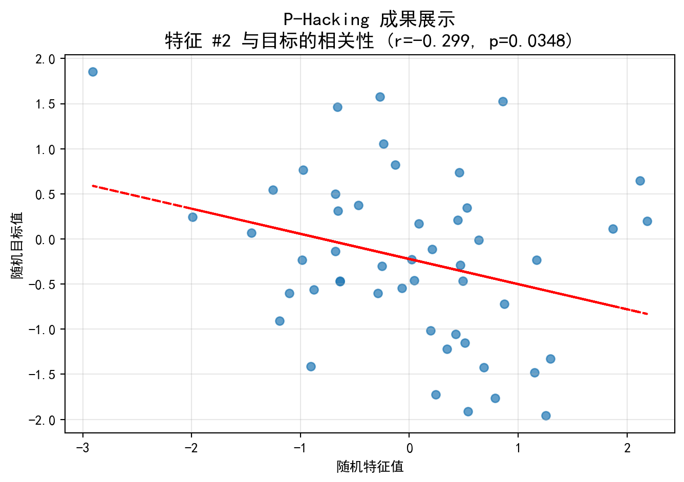
图 5.2 展示了在100个完全随机的特征中”精心挑选”出的一个”最佳”特征与目标变量的散点图。图中散点呈现出毫无规律的云状分布,但红色虚线的回归线却暗示了某种微弱的线性趋势。图表标题中的相关系数虽然不大(典型值在 \(|r| \approx 0.1\)–\(0.2\) 之间),但由于100个观测值的样本量,p值恰好低于0.05。这正是P值黑客的本质——在随机噪声中通过大量尝试”碰运气”式地发现虚假关联。如果一个量化基金将这个”发现”用于构建交易策略,其在样本外的表现几乎必然会回归至零。
图 5.2 presents a scatter plot of the “cherry-picked” best feature from among 100 entirely random features against the target variable. The scatter points exhibit a patternless cloud-like distribution, yet the red dashed regression line hints at a faint linear trend. Although the correlation coefficient in the chart title is small (typically \(|r| \approx 0.1\)–\(0.2\)), the p-value happens to fall below 0.05 thanks to the sample of 100 observations. This is the essence of P-hacking — discovering spurious associations through sheer trial-and-error in random noise. If a quantitative fund were to use this “discovery” to build a trading strategy, its out-of-sample performance would almost certainly revert to zero.
警示:当你看到一篇研究报告说”我们在分析了几百个财务指标后,发现指标X与股票超额收益有显著相关性”,请务必保持怀疑。这可能只是统计学上的”撞大运”——在足够多的指标中总会意外发现某个”显著”的结果。
Warning: When you see a research report claiming “after analyzing hundreds of financial indicators, we found that indicator X has a significant correlation with stock excess returns,” remain skeptical. This may simply be a statistical fluke — among enough indicators, some “significant” result will inevitably be found by chance.
5.3.2 2. 抽屉问题 (The File Drawer Problem)
为什么我们看到的科研论文大多是”成功”的(结果显著)?
- 因为那些”失败”的实验(P > 0.05)都被扔进抽屉里了,没人发表。
- 幸存者偏差:我们只看到了通过了显著性检验的幸存者,从而高估了效应的普遍性。
Why do most published scientific papers report “successful” (statistically significant) results?
- Because the “failed” experiments (P > 0.05) were tossed into file drawers and never published.
- Survivorship bias: We only see the survivors that passed the significance test, thus overestimating the prevalence of the effect. ## 假设检验 (Hypothesis Testing) {#sec-hypothesis-testing}
5.3.3 基本概念:惊讶度量与反证法 (Basic Concepts: Measuring Surprise and Proof by Contradiction)
假设检验基于反证法逻辑。我们先假设原假设 \(H_0\) 是对的(比如”银行ROE不高于2.5%“),然后看在这个假设下,我们的数据出现的可能性有多大。
Hypothesis testing is based on the logic of proof by contradiction. We first assume that the null hypothesis \(H_0\) is true (e.g., “the bank’s ROE does not exceed 2.5%”), and then examine how likely our observed data would be under this assumption.
如果数据出现的可能性极小(比如 \(p < 0.05\)),我们就会感到惊讶。这种惊讶迫使我们做出选择: 1. 发生了极小概率事件(运气爆棚)。 2. 原假设根本就是错的,所谓的”惊讶”其实是因为前提错了。
If the probability of the data occurring is extremely small (e.g., \(p < 0.05\)), we feel surprised. This surprise forces us to make a choice: 1. An extremely unlikely event has occurred (extraordinary luck). 2. The null hypothesis is simply wrong—the “surprise” is actually because the premise was incorrect.
科学推断倾向于后者,从而拒绝 \(H_0\)。这与法庭审判的逻辑——“无罪推定”直到”超越合理怀疑”——异曲同工。
Scientific inference favors the latter, leading us to reject \(H_0\). This is analogous to the logic of a court trial—“presumption of innocence” until “beyond reasonable doubt.”
5.3.3.1 假设的结构 (Structure of Hypotheses)
原假设(Null Hypothesis, \(H_0\)): 通常表示”无效应”、“无差异”或”现状”
Null Hypothesis (\(H_0\)): Typically represents “no effect,” “no difference,” or “the status quo”
备择假设(Alternative Hypothesis, \(H_1\) 或 \(H_a\)): 研究者希望证明的效应
Alternative Hypothesis (\(H_1\) or \(H_a\)): The effect the researcher hopes to demonstrate
如何设定假设?
How to formulate hypotheses?
原则: 将”希望证明”的陈述放在 \(H_1\) 中
Principle: Place the statement you “wish to prove” in \(H_1\)
例子1 (新量化策略更优):
- \(H_0\): 新量化策略与旧策略的年化收益率相同
- \(H_1\): 新量化策略比旧策略的年化收益率更高
Example 1 (A new quantitative strategy is superior):
- \(H_0\): The new quantitative strategy has the same annualized return as the old strategy
- \(H_1\): The new quantitative strategy has a higher annualized return than the old strategy
例子2 (检验上市公司财务违规率是否超标):
- \(H_0\): 上市公司财务违规率 ≤ 5%
- \(H_1\): 上市公司财务违规率 > 5%
Example 2 (Testing whether the financial fraud rate of listed companies exceeds the threshold):
- \(H_0\): The financial fraud rate of listed companies ≤ 5%
- \(H_1\): The financial fraud rate of listed companies > 5%
理由: 假设检验的设计使得如果拒绝 \(H_0\),我们有强证据支持 \(H_1\);但如果不能拒绝 \(H_0\),我们只是”没有足够证据”,而不是证明了 \(H_0\) 为真。
Rationale: The design of hypothesis testing ensures that if we reject \(H_0\), we have strong evidence supporting \(H_1\); however, if we fail to reject \(H_0\), we merely “lack sufficient evidence”—we have not proven \(H_0\) to be true.
5.3.3.2 两类错误 (Two Types of Errors)
| \(H_0\) 为真 | \(H_0\) 为假 | |
|---|---|---|
| 拒绝 \(H_0\) | 第一类错误(Type I Error) 假阳性(False Positive) 显著性水平 \(\alpha = P(\text{Type I})\) |
正确决策(True Positive) 功效(Power) = \(1-\beta\) |
| 不能拒绝 \(H_0\) | 正确决策(True Negative) | 第二类错误(Type II Error) 假阴性(False Negative) \(\beta = P(\text{Type II})\) |
| \(H_0\) is true | \(H_0\) is false | |
|---|---|---|
| Reject \(H_0\) | Type I Error False Positive Significance level \(\alpha = P(\text{Type I})\) |
Correct decision (True Positive) Power = \(1-\beta\) |
| Fail to reject \(H_0\) | Correct decision (True Negative) | Type II Error False Negative \(\beta = P(\text{Type II})\) |
经典权衡: 对于固定的样本量,减少 \(\alpha\) 会增加 \(\beta\),反之亦然。通常固定 \(\alpha\)(常用0.05或0.01),然后通过增大样本量来提高功效。
Classic trade-off: For a fixed sample size, decreasing \(\alpha\) increases \(\beta\), and vice versa. Typically, we fix \(\alpha\) (commonly at 0.05 or 0.01) and then increase the sample size to improve statistical power.
5.3.4 p值 (p-value)
定义: 在 \(H_0\) 为真的条件下,观测到当前样本(或更极端情况)的概率。
Definition: The probability of observing the current sample (or a more extreme outcome) given that \(H_0\) is true.
解读:
- p值 < \(\alpha\): 拒绝 \(H_0\) (结果显著)
- p值 ≥ \(\alpha\): 不能拒绝 \(H_0\) (结果不显著)
Interpretation:
- p-value < \(\alpha\): Reject \(H_0\) (result is statistically significant)
- p-value ≥ \(\alpha\): Fail to reject \(H_0\) (result is not statistically significant)
p值的常见误解
Common Misconceptions About p-values
❌ 错误: p值是 \(H_0\) 为真的概率 ✅ 正确: p值是在 \(H_0\) 为真时,得到当前数据的概率
❌ Incorrect: The p-value is the probability that \(H_0\) is true ✅ Correct: The p-value is the probability of obtaining the observed data given that \(H_0\) is true
❌ 错误: 小p值意味着 \(H_1\) 为真的概率大 ✅ 正确: 小p值说明数据与 \(H_0\) 不一致
❌ Incorrect: A small p-value means \(H_1\) is very likely true ✅ Correct: A small p-value indicates the data are inconsistent with \(H_0\)
❌ 错误: p < 0.05 表示发现了重要的、实用的效应 ✅ 正确: p值只衡量统计显著性,不衡量实际重要性。一个极小的p值可能来自一个统计显著但实际微不足道的效应
❌ Incorrect: p < 0.05 means a practically important effect has been discovered ✅ Correct: The p-value only measures statistical significance, not practical importance. An extremely small p-value may arise from an effect that is statistically significant but practically negligible
建议: 始终报告效应大小(如均值差、相关系数)和置信区间,而不仅仅是p值
Recommendation: Always report effect sizes (e.g., mean difference, correlation coefficient) and confidence intervals, not just p-values
5.3.5 单样本均值检验 (z检验与t检验) (One-Sample Mean Test: z-test and t-test)
检验假设: \[ H_0: \mu = \mu_0 \quad \text{vs} \quad H_1: \mu \neq \mu_0 \]
Test hypotheses: \[ H_0: \mu = \mu_0 \quad \text{vs} \quad H_1: \mu \neq \mu_0 \]
检验统计量如 式 5.8 所示:
The test statistic is shown in 式 5.8:
\[ t = \frac{\bar{X} - \mu_0}{S/\sqrt{n}} \sim t_{n-1} \quad (\text{under } H_0) \tag{5.8}\]
拒绝域: \(|t| > t_{\alpha/2, n-1}\) (双侧检验)
Rejection region: \(|t| > t_{\alpha/2, n-1}\) (two-sided test)
5.3.5.1 案例:检验工资水平 (Case Study: Testing Wage Levels)
什么是行业基准的假设检验?
What is hypothesis testing against an industry benchmark?
银行业是典型的高杠杆、强监管行业,其净资产收益率(ROE)长期以来是衡量银行经营效率的关键指标。行业分析师通常会设定一个「行业基准值」(如ROE达到10%),然后通过统计检验来判断某个子行业或区域的银行是否达到了这一基准。
The banking industry is a typical high-leverage, heavily regulated sector, where Return on Equity (ROE) has long served as a key indicator of operational efficiency. Industry analysts typically set an “industry benchmark” (e.g., ROE of 10%) and then use statistical tests to determine whether banks in a particular sub-sector or region meet this benchmark.
单样本t检验正是解决此类问题的标准工具:它将样本均值与一个已知的基准值进行比较,在考虑了样本波动性的情况下,判断总体均值是否与基准值存在统计上的显著差异。下面使用本地财务数据对长三角银行行业的平均ROE进行单样本t检验,结果如 表 5.4 所示。
The one-sample t-test is the standard tool for such problems: it compares the sample mean against a known benchmark value and, after accounting for sampling variability, determines whether the population mean differs significantly from the benchmark. Below, we perform a one-sample t-test on the average ROE of the Yangtze River Delta banking industry using local financial data. The results are shown in 表 5.4.
# ========== 导入所需库 ==========
# ========== Import required libraries ==========
import numpy as np               # 数值计算库
# NumPy library for numerical computation
from scipy import stats          # 统计检验模块,提供t分布函数
# SciPy stats module providing t-distribution functions
import pandas as pd              # 数据分析库,用于读取和处理HDF5数据
# Pandas library for reading and processing HDF5 data
from pathlib import Path         # 路径处理模块,跨平台兼容
# Path module for cross-platform file path handling

# ========== 第1步:加载本地数据 ==========
# ========== Step 1: Load local data ==========
import platform  # 导入平台检测模块,用于判断操作系统
# Import platform module to detect the operating system
if platform.system() == 'Windows':  # Windows系统数据路径
    # Windows system data path
    data_directory_path = Path('C:/qiufei/data/stock')  # Windows本地数据路径
    # Local data path for Windows
else:  # Linux系统数据路径
    # Linux system data path
    data_directory_path = Path('/home/ubuntu/r2_data_mount/qiufei/data/stock')  # Linux本地数据路径
    # Local data path for Linux
basic_info_dataframe = pd.read_hdf(data_directory_path / 'stock_basic_data.h5')       # 读取上市公司基本信息
# Read basic information of listed companies
financial_statement_dataframe = pd.read_hdf(data_directory_path / 'financial_statement.h5')  # 读取财务报表数据
# Read financial statement data

# ========== 第2步:数据筛选——锁定长三角银行业上市公司 ==========
# ========== Step 2: Data filtering — Identify YRD banking listed companies ==========
yrd_provinces_list = ['上海市', '江苏省', '浙江省', '安徽省']  # 定义长三角四省市
# Define the four YRD provinces/municipalities
target_industry_name = '货币金融服务'   # 国统局行业分类中的银行业名称
# Banking industry name in the NBS industry classification
target_quarter_string = '2023q3'        # 选取2023年第三季度作为分析时点
# Select Q3 2023 as the analysis period

# 构建布尔筛选条件:省份在长三角范围内
# Build boolean filter: province within the YRD region
region_mask = basic_info_dataframe['province'].isin(yrd_provinces_list)  # 构建地区筛选布尔掩码
# Create a boolean mask for region filtering
# 构建布尔筛选条件:行业为银行业
# Build boolean filter: industry is banking
industry_mask = basic_info_dataframe['industry_name'] == target_industry_name  # 筛选货币金融服务行业
# Filter for the monetary and financial services industry
# 取交集:同时满足地区和行业条件的公司
# Take the intersection: companies satisfying both region and industry criteria
target_companies_dataframe = basic_info_dataframe[region_mask & industry_mask]  # 长三角银行业公司
# YRD banking companies
长三角银行业上市公司筛选完成。下面获取指定季度的财务数据,计算ROE并进行异常值处理。
The filtering of YRD banking listed companies is complete. Next, we retrieve the financial data for the specified quarter, calculate ROE, and handle outliers.
# ========== 第3步:获取指定季度的财务数据并计算ROE ==========
# ========== Step 3: Retrieve quarterly financial data and calculate ROE ==========
# 从财务报表中筛选目标季度的净利润和股东权益数据
# Filter the target quarter's net profit and total equity from financial statements
financial_statement_quarter_dataframe = financial_statement_dataframe[  # 从财务报表筛选目标季度数据
    # Filter target quarter data from financial statements
    financial_statement_dataframe['quarter'] == target_quarter_string   # 筛选2023Q3数据
    # Filter for Q3 2023 data
][['order_book_id', 'net_profit', 'total_equity']]                     # 只保留需要的三列
# Keep only the three required columns

# 将公司基本信息与财务数据按股票代码合并
# Merge company basic information with financial data by stock code
merged_analysis_dataframe = pd.merge(  # 内连接合并两张表
    # Inner join to merge two tables
    target_companies_dataframe,              # 左表:目标公司列表
    # Left table: list of target companies
    financial_statement_quarter_dataframe,    # 右表:财务数据
    # Right table: financial data
    on='order_book_id',                      # 合并键:股票代码
    # Merge key: stock code
    how='inner'                              # 内连接:只保留两表都有的记录
    # Inner join: keep only records present in both tables
)

# 计算ROE(净资产收益率)= 净利润 / 股东权益
# Calculate ROE (Return on Equity) = Net Profit / Total Equity
merged_analysis_dataframe['roe'] = merged_analysis_dataframe['net_profit'] / merged_analysis_dataframe['total_equity']  # 计算ROE=净利润/股东权益
# Compute ROE = net profit / total equity

# ========== 第4步:异常值处理——去除极端ROE ==========
# ========== Step 4: Outlier handling — Remove extreme ROE values ==========
# 银行ROE通常较稳定,但防止极端分母导致的异常值
# Bank ROE is typically stable, but extreme denominators may cause outliers
clean_analysis_dataframe = merged_analysis_dataframe[  # 筛选ROE合理范围内的样本
    # Filter samples within a reasonable ROE range
    (merged_analysis_dataframe['roe'] > -0.5) &   # ROE > -50%(排除极端亏损)
    # ROE > -50% (exclude extreme losses)
    (merged_analysis_dataframe['roe'] < 0.5)       # ROE < 50%(排除异常高值)
    # ROE < 50% (exclude abnormally high values)
]

roe_sample_series = clean_analysis_dataframe['roe']  # 提取清洗后的ROE序列
# Extract the cleaned ROE series
sample_size_n = len(roe_sample_series)                # 计算样本量
# Calculate the sample size
数据清洗完毕,长三角银行业上市公司的ROE样本已生成。下面设定假设检验参数,执行单样本t检验,并计算总体均值的95%置信区间,以判断该行业平均季度ROE是否显著高于2.5%(对应年化约10%)。
Data cleaning is complete, and the ROE sample for YRD banking listed companies has been generated. Next, we set the hypothesis test parameters, perform the one-sample t-test, and compute the 95% confidence interval for the population mean to determine whether the industry’s average quarterly ROE is significantly above 2.5% (approximately 10% annualized).
# ========== 第5步:设定假设检验参数 ==========
# ========== Step 5: Set hypothesis test parameters ==========
# H0: μ ≤ 0.025 (长三角银行业季度ROE不超过2.5%,对应年化约10%)
# H0: μ ≤ 0.025 (YRD banking quarterly ROE does not exceed 2.5%, ~10% annualized)
# H1: μ > 0.025 (季度ROE显著高于2.5%)
# H1: μ > 0.025 (quarterly ROE is significantly above 2.5%)
# 这是一个右侧单尾检验
# This is a right-tailed one-sided test
null_hypothesis_mean_value = 0.025   # 原假设下的总体均值μ₀ = 2.5%
# Null hypothesis population mean μ₀ = 2.5%
significance_level_alpha = 0.05      # 显著性水平α = 5%
# Significance level α = 5%

# ========== 第6步:计算检验统计量 ==========
# ========== Step 6: Calculate the test statistic ==========
sample_mean_roe = roe_sample_series.mean()       # 样本均值 x̄
# Sample mean x̄
sample_standard_deviation = roe_sample_series.std()  # 样本标准差 s(默认ddof=1,即Bessel修正)
# Sample standard deviation s (default ddof=1, i.e., Bessel's correction)
# t统计量 = (x̄ - μ₀) / (s / √n),衡量样本均值偏离原假设值的标准误数
# t-statistic = (x̄ - μ₀) / (s / √n), measuring how many standard errors the sample mean deviates from the null value
t_statistic_value = (sample_mean_roe - null_hypothesis_mean_value) / (sample_standard_deviation / np.sqrt(sample_size_n))  # 计算t统计量
# Calculate the t-statistic

# ========== 第7步:计算p值(右侧单尾) ==========
# ========== Step 7: Calculate the p-value (right-tailed) ==========
# p = P(T > t_obs | H0为真),即在原假设下观测到比当前t值更极端结果的概率
# p = P(T > t_obs | H0 is true), the probability of observing a more extreme result under H0
calculated_p_value_right_tail = 1 - stats.t.cdf(t_statistic_value, df=sample_size_n - 1)  # 右侧单尾p值
# Right-tailed one-sided p-value

# ========== 第8步:计算95%双侧置信区间(辅助参考) ==========
# ========== Step 8: Calculate the 95% two-sided confidence interval (supplementary reference) ==========
# 虽然本检验为单侧,但双侧CI有助于直观展示参数的合理范围
# Although this is a one-sided test, the two-sided CI helps visualize the plausible range of the parameter
# CI下界 = x̄ - t_{0.975, n-1} × (s / √n)
# CI lower bound = x̄ - t_{0.975, n-1} × (s / √n)
confidence_interval_lower_bound = sample_mean_roe - stats.t.ppf(0.975, sample_size_n - 1) * sample_standard_deviation / np.sqrt(sample_size_n)  # CI下界
# CI lower bound
# CI上界 = x̄ + t_{0.975, n-1} × (s / √n)
# CI upper bound = x̄ + t_{0.975, n-1} × (s / √n)
confidence_interval_upper_bound = sample_mean_roe + stats.t.ppf(0.975, sample_size_n - 1) * sample_standard_deviation / np.sqrt(sample_size_n)  # CI上界
# CI upper bound
检验统计量和置信区间计算完毕。下面输出完整的假设检验报告。
The test statistic and confidence interval calculations are complete. Below, we output the full hypothesis testing report.
# ========== 第9步:输出完整检验报告 ==========
# ========== Step 9: Output the complete test report ==========
print(f'行业: 长三角{target_industry_name}')       # 打印行业范围
# Print the industry scope
print(f'假设检验目标:')                              # 打印假设结构
# Print hypothesis structure
print(f'  H0: 平均季度ROE ≤ {null_hypothesis_mean_value:.1%} (年化约10%)')   # 原假设
# Null hypothesis
print(f'  H1: 平均季度ROE > {null_hypothesis_mean_value:.1%}')               # 备择假设
# Alternative hypothesis
print(f'  显著性水平: α = {significance_level_alpha}')                        # 显著性水平
# Significance level

print(f'\n样本统计量:')                              # 分隔:样本描述统计
# Section separator: sample descriptive statistics
print(f'  样本量: n = {sample_size_n}')              # 有效样本量
# Effective sample size
print(f'  样本均值: x̄ = {sample_mean_roe:.4f} = {sample_mean_roe:.2%}')  # 均值(小数+百分比)
# Mean (decimal + percentage)
print(f'  样本标准差: s = {sample_standard_deviation:.4f}')               # 标准差
# Standard deviation

print(f'\n检验结果:')                                # 分隔:核心检验结论
# Section separator: core test conclusions
print(f'  检验统计量: t = {t_statistic_value:.4f}')  # t统计量
# t-statistic
print(f'  p值 (单侧): {calculated_p_value_right_tail:.6f}')  # 右侧p值
# Right-tailed p-value

print(f'\n结论:')                                    # 分隔:最终判断
# Section separator: final conclusion
if calculated_p_value_right_tail < significance_level_alpha:  # 若p < α则拒绝H0
    # If p < α, reject H0
    print(f'  拒绝 H0。有充分证据表明长三角银行业平均季度ROE显著高于{null_hypothesis_mean_value:.1%}。')  # 拒绝原假设的结论
    # Conclusion of rejecting the null hypothesis
else:                                                          # 否则不能拒绝H0
    # Otherwise, fail to reject H0
    print(f'  不能拒绝 H0。没有足够证据表明长三角银行业平均季度ROE显著高于{null_hypothesis_mean_value:.1%}。')  # 不拒绝的结论
    # Conclusion of failing to reject H0

print(f'\n95%置信区间 (均值): [{confidence_interval_lower_bound:.2%}, {confidence_interval_upper_bound:.2%}]')  # CI范围
# 95% confidence interval range
print(f'注意: 样本量较小时需谨慎解释,但银行业通常样本量有限。')  # 提示小样本注意事项
# Note on small sample size considerations
行业: 长三角货币金融服务
假设检验目标:
H0: 平均季度ROE ≤ 2.5% (年化约10%)
H1: 平均季度ROE > 2.5%
显著性水平: α = 0.05
样本统计量:
样本量: n = 18
样本均值: x̄ = 0.0854 = 8.54%
样本标准差: s = 0.0186
检验结果:
检验统计量: t = 13.8137
p值 (单侧): 0.000000
结论:
拒绝 H0。有充分证据表明长三角银行业平均季度ROE显著高于2.5%。
95%置信区间 (均值): [7.62%, 9.46%]
注意: 样本量较小时需谨慎解释,但银行业通常样本量有限。表 5.4 展示了长三角银行业平均ROE的单样本t检验结果。样本包含18家银行,样本均值为8.54%,样本标准差为1.86%。在单侧检验(\(H_1: \mu > 2.5\%\))下,t统计量高达13.8137,对应p值为0.000000(远小于0.05),因此在5%显著性水平下拒绝原假设,有充分证据表明长三角银行业平均季度ROE显著高于2.5%的基准值。95%置信区间为[7.62%, 9.46%],该区间完全位于2.5%基准之上,从另一个角度印证了检验结论。值得注意的是,样本量仅为18家(银行业上市公司数量本身有限),因此使用t分布(而非正态分布)进行小样本推断是恰当的选择。8.54%的季度ROE折合年化约34%,显示银行业整体盈利能力较强。
表 5.4 presents the results of the one-sample t-test on the average ROE of the YRD banking industry. The sample contains 18 banks with a sample mean of 8.54% and a sample standard deviation of 1.86%. Under the one-sided test (\(H_1: \mu > 2.5\%\)), the t-statistic reaches 13.8137 with a p-value of 0.000000 (far below 0.05). Therefore, at the 5% significance level, we reject the null hypothesis, with sufficient evidence that the average quarterly ROE of YRD banks is significantly above the 2.5% benchmark. The 95% confidence interval is [7.62%, 9.46%], lying entirely above the 2.5% benchmark, corroborating the test conclusion from another perspective. It is noteworthy that the sample size is only 18 (the number of publicly listed banks is inherently limited), making the use of the t-distribution (rather than the normal distribution) an appropriate choice for small-sample inference. The 8.54% quarterly ROE translates to approximately 34% annualized, indicating strong overall profitability in the banking industry.
5.3.6 两样本均值检验 (Two-Sample Mean Test)
独立样本t检验: 比较两个独立总体的均值。检验统计量如 式 7.2 所示:
Independent samples t-test: Compares the means of two independent populations. The test statistic is shown in 式 7.2:
\[ t = \frac{\bar{X}_1 - \bar{X}_2}{S_p\sqrt{\frac{1}{n_1} + \frac{1}{n_2}}} \sim t_{n_1+n_2-2} \tag{5.9}\]
其中合并标准差的计算公式如 式 5.10 所示:
where the pooled standard deviation is calculated as shown in 式 5.10:
\[ S_p = \sqrt{\frac{(n_1-1)S_1^2 + (n_2-1)S_2^2}{n_1+n_2-2}} \tag{5.10}\]
配对样本t检验: 比较配对数据的均值差异,检验统计量如 式 7.3 所示:
Paired samples t-test: Compares the mean difference of paired data. The test statistic is shown in 式 7.3:
\[ t = \frac{\bar{d}}{S_d/\sqrt{n}} \sim t_{n-1} \tag{5.11}\]
其中 \(d_i = X_{1i} - X_{2i}\) 是配对差值。
where \(d_i = X_{1i} - X_{2i}\) is the paired difference.
5.3.6.1 案例:A/B测试效果评估 (Case Study: A/B Test Evaluation)
什么是区域经济差异的双样本比较?
What is a two-sample comparison of regional economic differences?
在区域经济研究和投资策略中,比较不同地区企业的经营绩效差异是一个常见且重要的分析任务。例如,上海作为长三角的核心城市和中国的金融中心,其上市公司的ROE是否显著高于安徽省?这种区域差异对于跨区域资产配置和产业布局决策至关重要。
In regional economic research and investment strategy, comparing the operational performance of enterprises across different regions is a common and important analytical task. For instance, as the core city of the Yangtze River Delta and China’s financial center, does Shanghai’s listed companies have significantly higher ROE than those in Anhui Province? Such regional differences are crucial for cross-regional asset allocation and industrial layout decisions.
双样本t检验是比较两个独立群体均值差异的经典统计方法。它不仅能告诉我们两组样本均值是否存在差异,更重要的是能在控制抽样误差的前提下,判断这种差异是否具有统计显著性。下面我们通过对比上海与安徽两地上市公司的平均ROE来演示双样本t检验,结果如 表 5.5 所示。
The two-sample t-test is a classic statistical method for comparing the mean difference between two independent groups. It not only tells us whether there is a difference in sample means but, more importantly, determines whether this difference is statistically significant after controlling for sampling error. Below, we demonstrate the two-sample t-test by comparing the average ROE of listed companies in Shanghai and Anhui. The results are shown in 表 5.5.
import numpy as np  # 数值计算库
# NumPy library for numerical computation
from scipy import stats  # 统计检验模块
# SciPy stats module for statistical testing
import pandas as pd  # 数据分析库
# Pandas library for data analysis
from pathlib import Path  # 路径处理模块
# Path module for file path handling

# ========== 导入所需库 ==========
# ========== Import required libraries ==========
import numpy as np               # 数值计算库
# NumPy library for numerical computation
from scipy import stats          # 统计检验模块
# SciPy stats module for statistical testing
import pandas as pd              # 数据分析库
# Pandas library for data analysis
from pathlib import Path         # 路径处理模块
# Path module for file path handling

# ========== 第1步:加载本地数据 ==========
# ========== Step 1: Load local data ==========
import platform  # 导入平台检测模块,用于判断操作系统
# Import platform module to detect the operating system
if platform.system() == 'Windows':  # Windows系统数据路径
    # Windows system data path
    data_directory_path = Path('C:/qiufei/data/stock')  # Windows本地数据路径
    # Local data path for Windows
else:  # Linux系统数据路径
    # Linux system data path
    data_directory_path = Path('/home/ubuntu/r2_data_mount/qiufei/data/stock')  # Linux本地数据路径
    # Local data path for Linux
basic_info_dataframe = pd.read_hdf(data_directory_path / 'stock_basic_data.h5')       # 读取公司基本信息
# Read company basic information
financial_statement_dataframe = pd.read_hdf(data_directory_path / 'financial_statement.h5')  # 读取财务报表
# Read financial statements
数据加载完毕。下面按地区筛选上海与安徽的上市公司并提取财务数据。
Data loading is complete. Next, we filter listed companies in Shanghai and Anhui by region and extract the financial data.
# ========== 第2步:按地区分组筛选公司 ==========
# ========== Step 2: Filter companies by region ==========
target_quarter_string = '2023q3'                                       # 目标季度
# Target quarter

# 创建布尔掩码:分别筛选上海和安徽的上市公司
# Create boolean masks: filter listed companies in Shanghai and Anhui respectively
shanghai_companies_mask = basic_info_dataframe['province'] == '上海市'  # 上海公司掩码
# Boolean mask for Shanghai companies
anhui_companies_mask = basic_info_dataframe['province'] == '安徽省'     # 安徽公司掩码
# Boolean mask for Anhui companies
shanghai_companies_dataframe = basic_info_dataframe[shanghai_companies_mask]  # 提取上海公司
# Extract Shanghai companies
anhui_companies_dataframe = basic_info_dataframe[anhui_companies_mask]        # 提取安徽公司
# Extract Anhui companies

# ========== 第3步:获取指定季度的财务数据 ==========
# ========== Step 3: Retrieve financial data for the specified quarter ==========
# 从财务报表中筛选2023Q3的净利润和股东权益
# Filter Q3 2023 net profit and total equity from financial statements
financial_statement_quarter_dataframe = financial_statement_dataframe[  # 从财务报表筛选目标季度
    # Filter the target quarter from financial statements
    financial_statement_dataframe['quarter'] == target_quarter_string   # 筛选目标季度
    # Filter for the target quarter
][['order_book_id', 'net_profit', 'total_equity']]                     # 只保留关键列
# Keep only the key columns
基础数据加载与地区筛选完成。下面定义ROE计算函数并分别计算上海与安徽两地上市公司的净资产收益率。
Basic data loading and regional filtering are complete. Next, we define the ROE calculation function and compute the return on equity for listed companies in Shanghai and Anhui respectively.
# ========== 第4步:定义ROE清洗函数 ==========
# ========== Step 4: Define the ROE cleaning function ==========
def calculate_cleaned_roe(companies_df, financials_df):  # 定义ROE计算与清洗函数
    # Define the ROE calculation and cleaning function
    """
    计算并清洗公司ROE(净资产收益率)。
    步骤:合并数据 → 计算ROE → 去除无穷值/空值 → 分位数去极值(1%-99%)。

    参数:
        companies_df: 包含公司基本信息的DataFrame
        financials_df: 包含财务数据的DataFrame
    返回:
        清洗后的ROE Series
    """
    merged_df = pd.merge(companies_df, financials_df, on='order_book_id', how='inner')  # 按股票代码合并
    # Merge by stock code
    merged_df['roe'] = merged_df['net_profit'] / merged_df['total_equity']  # 计算ROE = 净利润/股东权益
    # Calculate ROE = net profit / total equity
    # 清洗第一步:将无穷值替换为NaN,然后删除含NaN的行
    # Cleaning step 1: Replace infinity values with NaN, then drop rows containing NaN
    merged_df = merged_df.replace([np.inf, -np.inf], np.nan).dropna(subset=['roe'])  # 将无穷大值替换为NaN并删除空值
    # Replace infinity with NaN and drop null values
    # 清洗第二步:计算1%和99%分位数阈值,Winsorize去极端值
    # Cleaning step 2: Compute 1st and 99th percentile thresholds, Winsorize to remove extreme values
    # 这样可以避免少数壳股或ST公司的极端ROE干扰均值对比
    # This prevents extreme ROE values from a few shell or ST companies from distorting the mean comparison
    quantile_low_threshold = merged_df['roe'].quantile(0.01)    # 下限:1%分位数
    # Lower bound: 1st percentile
    quantile_high_threshold = merged_df['roe'].quantile(0.99)   # 上限:99%分位数
    # Upper bound: 99th percentile
    return merged_df[  # 返回去极值后的ROE序列
        # Return the ROE series after removing extreme values
        (merged_df['roe'] >= quantile_low_threshold) &          # 大于等于下限
        # Greater than or equal to the lower bound
        (merged_df['roe'] <= quantile_high_threshold)           # 小于等于上限
        # Less than or equal to the upper bound
    ]['roe']                                                     # 返回清洗后的ROE序列
    # Return the cleaned ROE series

# ========== 第5步:分别计算两地的清洗后ROE ==========
# ========== Step 5: Calculate cleaned ROE for both regions ==========
shanghai_roe_series = calculate_cleaned_roe(shanghai_companies_dataframe, financial_statement_quarter_dataframe)  # 上海ROE
# Shanghai ROE
anhui_roe_series = calculate_cleaned_roe(anhui_companies_dataframe, financial_statement_quarter_dataframe)        # 安徽ROE
# Anhui ROE
两地区上市公司的清洗后ROE数据已准备就绪。下面计算描述性统计量,执行Welch’s t检验,并计算均值差的95%置信区间,以判断上海与安徽上市公司的平均盈利能力是否存在显著差异。
The cleaned ROE data for listed companies in both regions is ready. Next, we calculate descriptive statistics, perform Welch’s t-test, and compute the 95% confidence interval for the mean difference to determine whether there is a significant difference in average profitability between Shanghai and Anhui listed companies.
# ========== 第6步:计算描述性统计量 ==========
# ========== Step 6: Calculate descriptive statistics ==========
shanghai_sample_size = len(shanghai_roe_series)     # 上海样本量
# Shanghai sample size
anhui_sample_size = len(anhui_roe_series)           # 安徽样本量
# Anhui sample size
shanghai_sample_mean = shanghai_roe_series.mean()   # 上海样本均值
# Shanghai sample mean
anhui_sample_mean = anhui_roe_series.mean()         # 安徽样本均值
# Anhui sample mean
shanghai_sample_std = shanghai_roe_series.std()     # 上海样本标准差
# Shanghai sample standard deviation
anhui_sample_std = anhui_roe_series.std()           # 安徽样本标准差
# Anhui sample standard deviation

# ========== 第7步:执行Welch's t检验(不假设方差相等) ==========
# ========== Step 7: Perform Welch's t-test (does not assume equal variances) ==========
# Welch's t-test比Student's t-test更稳健,不要求两组方差相等
# Welch's t-test is more robust than Student's t-test and does not require equal variances
# equal_var=False 指定使用Welch近似自由度
# equal_var=False specifies using Welch's approximate degrees of freedom
t_statistic_value, p_value_two_sided = stats.ttest_ind(  # 执行Welch's t检验
    # Perform Welch's t-test
    shanghai_roe_series, anhui_roe_series, equal_var=False  # 双侧检验,返回t值和p值
    # Two-sided test, returns t-value and p-value
)

# ========== 第8步:计算均值差的95%置信区间 ==========
# ========== Step 8: Calculate the 95% confidence interval for the mean difference ==========
# 差异的标准误 SE = sqrt(s1²/n1 + s2²/n2)
# Standard error of the difference SE = sqrt(s1²/n1 + s2²/n2)
standard_error_difference = np.sqrt(shanghai_sample_std**2 / shanghai_sample_size + anhui_sample_std**2 / anhui_sample_size)  # 差异的标准误 SE
# Standard error of the difference
mean_difference = shanghai_sample_mean - anhui_sample_mean  # 均值差 = x̄₁ - x̄₂
# Mean difference = x̄₁ - x̄₂
z_critical_value_975 = stats.norm.ppf(0.975)                # z_{0.975} ≈ 1.96(大样本近似)
# z_{0.975} ≈ 1.96 (large-sample approximation)
# CI = (x̄₁ - x̄₂) ± z_{0.975} × SE
# CI = (x̄₁ - x̄₂) ± z_{0.975} × SE
confidence_interval_lower_bound = mean_difference - z_critical_value_975 * standard_error_difference  # CI下界
# CI lower bound
confidence_interval_upper_bound = mean_difference + z_critical_value_975 * standard_error_difference  # CI上界
# CI upper bound
描述性统计量计算、Welch t检验和置信区间计算完毕。下面输出完整检验报告。
Descriptive statistics, the Welch t-test, and confidence interval calculations are complete. Below, we output the full test report.
# ========== 第9步:输出检验报告 ==========
# ========== Step 9: Output the test report ==========
print(f'分组对比:')                                                           # 标题
# Title
print(f'  组1 (上海): n={shanghai_sample_size}, 均值={shanghai_sample_mean:.2%}, 标准差={shanghai_sample_std:.2%}')  # 上海统计量
# Shanghai statistics
print(f'  组2 (安徽): n={anhui_sample_size}, 均值={anhui_sample_mean:.2%}, 标准差={anhui_sample_std:.2%}')          # 安徽统计量
# Anhui statistics
print(f'  均值差异: {mean_difference:.4f} = {mean_difference:.2%}')           # 均值差
# Mean difference

print(f'\n假设检验:')                                                         # 假设结构
# Hypothesis structure
print(f'  H0: μ_上海 = μ_安徽')                                               # 原假设:两地均值相等
# Null hypothesis: the two regional means are equal
print(f'  H1: μ_上海 ≠ μ_安徽')                                               # 备择假设:两地均值不等
# Alternative hypothesis: the two regional means are not equal
print(f'  检验结果: t={t_statistic_value:.4f}, p={p_value_two_sided:.4f}')    # 输出t值和p值
# Output t-value and p-value

significance_level_alpha = 0.05                                               # 设定显著性水平
# Set significance level
if p_value_two_sided < significance_level_alpha:                              # 若p < α,拒绝H0
    # If p < α, reject H0
    print(f'\n结论: 拒绝 H0 (p < {significance_level_alpha})。上海与安徽上市公司在该季度的平均ROE存在显著差异。')  # 拒绝H0的结论
    # Conclusion: reject H0
else:                                                                          # 否则不能拒绝H0
    # Otherwise, fail to reject H0
    print(f'\n结论: 不能拒绝 H0 (p ≥ {significance_level_alpha})。没有足够证据表明两地上市公司平均ROE有显著差异。')  # 不拒绝的结论
    # Conclusion: fail to reject H0

print(f'\n均值差的95%置信区间: [{confidence_interval_lower_bound:.2%}, {confidence_interval_upper_bound:.2%}]')  # 输出CI
# Output the 95% confidence interval for the mean difference
分组对比:
组1 (上海): n=425, 均值=3.72%, 标准差=5.85%
组2 (安徽): n=168, 均值=4.81%, 标准差=6.25%
均值差异: -0.0108 = -1.08%
假设检验:
H0: μ_上海 = μ_安徽
H1: μ_上海 ≠ μ_安徽
检验结果: t=-1.9340, p=0.0541
结论: 不能拒绝 H0 (p ≥ 0.05)。没有足够证据表明两地上市公司平均ROE有显著差异。
均值差的95%置信区间: [-2.18%, 0.01%]表 5.5 展示了上海与安徽上市公司平均ROE的对比检验结果。上海组共425家公司,平均ROE为3.72%(标准差5.85%);安徽组共168家公司,平均ROE为4.81%(标准差6.25%)。安徽的平均ROE反而高出上海约1.08个百分点。Welch t检验的t统计量为-1.9340,双侧p值为0.0541,恰好略高于0.05的显著性水平,因此不能拒绝原假设——没有足够证据表明两地上市公司的平均ROE存在显著差异。均值差的95%置信区间为[-2.18%, 0.01%],该区间包含了零值(上界恰好为0.01%),与不拒绝的结论一致。这是一个典型的”边界案例”:p值距离临界值仅差0.004,提醒我们0.05并非一个绝对的”神奇门槛”,而是一个人为设定的决策标准。从经济角度看,两地企业均为长三角核心区域,产业结构和市场环境有较多相似之处,ROE差异不显著是合理的。
表 5.5 presents the comparative test results of average ROE between Shanghai and Anhui listed companies. The Shanghai group consists of 425 companies with an average ROE of 3.72% (standard deviation 5.85%); the Anhui group consists of 168 companies with an average ROE of 4.81% (standard deviation 6.25%). Anhui’s average ROE is actually about 1.08 percentage points higher than Shanghai’s. The Welch t-test yields a t-statistic of -1.9340 with a two-sided p-value of 0.0541, just slightly above the 0.05 significance level. Therefore, we fail to reject the null hypothesis—there is insufficient evidence to conclude that the average ROE of listed companies in the two regions differs significantly. The 95% confidence interval for the mean difference is [-2.18%, 0.01%], which contains zero (the upper bound is exactly 0.01%), consistent with the failure to reject. This is a classic “borderline case”: the p-value is only 0.004 away from the critical value, reminding us that 0.05 is not an absolute “magic threshold” but rather an arbitrarily set decision criterion. From an economic perspective, enterprises in both regions belong to the core of the Yangtze River Delta, sharing similar industrial structures and market environments, making the lack of significant ROE difference a reasonable finding.
4. “热手谬误” (The Hot Hand Fallacy)
- 篮球迷常说:“这名球员手感火热,下一球肯定进!”
- 统计真相:对大多数球员来说,投篮命中只是一个独立的伯努利试验。连续三次命中后,第四次命中的概率并不比平时高。
- 为什么我们会有这种错觉? 人类的大脑擅长在随机序列中寻找模式(Pattern Seeking)。我们把连续发生的随机事件误认为是有因果关系的。
- 实证任务:下载NBA某位球星的逐球数据(Play-by-play),计算他在连续命中3球后的命中率,是否显著高于他的平均命中率?
4. “The Hot Hand Fallacy”
- Basketball fans often say: “This player is on fire—the next shot will definitely go in!”
- Statistical truth: For most players, each shot is simply an independent Bernoulli trial. After three consecutive makes, the probability of making the fourth shot is no higher than usual.
- Why do we have this illusion? The human brain excels at seeking patterns in random sequences (Pattern Seeking). We mistake consecutively occurring random events for causally related ones.
- Empirical exercise: Download play-by-play data for an NBA star and calculate his shooting percentage after three consecutive makes—is it significantly higher than his overall average?
5. 均值回归 (Regression to the Mean)
- 为什么高考状元在大学阶段往往表现平平?
- 为什么”双十一”创下销售纪录的店铺次年同期往往难以复制辉煌?
- 这不是诅咒,这是统计学的必然。
- 极端的表现(无论是极好还是极差)通常是由”能力 + 极好的运气”构成的。
- 运气是不可持续的。当运气回归正常时,表现自然会回落到平均水平。
- 商业启示:不要因为某位销售员上季度业绩翻倍就盲目提拔他,那可能只是运气。
5. Regression to the Mean
- Why do top scorers on the college entrance exam often perform unremarkably in university?
- Why do online stores that set sales records during “Double Eleven” often struggle to replicate their glory the following year?
- This is not a curse—it is a statistical inevitability.
- Extreme performance (whether exceptionally good or bad) is typically composed of “ability + exceptionally good luck.”
- Luck is unsustainable. When luck reverts to normal, performance naturally falls back to the average.
- Business insight: Do not blindly promote a salesperson just because their performance doubled last quarter—it may have been mere luck. ## 启发式思考题 (Heuristic Problems) {#sec-heuristic-problems}
本节提供一些开放性的思考题,旨在连接理论与现实世界的复杂性。
This section presents a set of open-ended discussion questions designed to bridge theory and the complexity of the real world.
1. “p值黑客” (p-hacking) 的反思 假设你是一个量化分析师,你手头有 100 个不同的财务指标。你试图找出哪个指标能预测明天的股价涨跌。你对每个指标都做了一次相关性检验。
1. Reflections on “p-Hacking” Suppose you are a quantitative analyst with 100 different financial indicators at your disposal. You are trying to find which indicator can predict tomorrow’s stock price movement. You run a correlation test on each indicator.
即使这 100 个指标全都是毫无意义的随机噪声,你大概率会发现多少个 p < 0.05 的”显著”指标?
计算发现至少一个”显著”指标的概率:\(1 - (0.95)^{100}\)。这对你的投资策略意味着什么?
实现任务:编写一个 Python 脚本模拟这个过程,生成 100 列随机数据和 1 列随机目标,进行相关性筛选,看看能筛出多少”伪圣杯”。
Even if all 100 indicators are nothing but meaningless random noise, how many “significant” indicators with p < 0.05 would you expect to find?
Calculate the probability of finding at least one “significant” indicator: \(1 - (0.95)^{100}\). What does this imply for your investment strategy?
Implementation task: Write a Python script to simulate this process—generate 100 columns of random data and 1 column of random target, then screen for correlations to see how many “false holy grails” emerge.
参考答案:
Reference Answer:
如 图 5.3 所示,即使所有指标都是纯随机噪声,仍有约5%的指标会通过显著性检验。
As shown in 图 5.3, even when all indicators are pure random noise, approximately 5% of them will still pass the significance test.
# ========== 导入所需库 ==========
# ========== Import required libraries ==========
import numpy as np               # 数值计算库
# Import NumPy for numerical computation
from scipy import stats          # 统计检验模块
# Import the stats module from SciPy for statistical tests
import matplotlib.pyplot as plt  # 绘图库
# Import Matplotlib for plotting

# ========== 中文字体配置 ==========
# ========== Chinese font configuration ==========
plt.rcParams['font.sans-serif'] = ['SimHei']        # 使用黑体显示中文
# Use SimHei font for Chinese character display
plt.rcParams['axes.unicode_minus'] = False           # 修复负号显示
# Fix the display of minus signs

np.random.seed(42)  # 设定随机种子以保证结果可复现
# Set random seed for reproducibility

# ========== 第1步:设定蒙特卡洛模拟参数 ==========
# ========== Step 1: Set Monte Carlo simulation parameters ==========
number_of_indicators = 100      # 每次模拟测试100个随机财务指标
# Test 100 random financial indicators per simulation
sample_size = 200               # 每个指标有200个"交易日"的观测值
# Each indicator has 200 "trading day" observations
number_of_simulations = 1000    # 总共重复模拟1000次
# Repeat the simulation 1000 times in total
蒙特卡洛模拟参数设定完毕。下面执行1000次模拟,每次对100个纯噪声指标进行相关性检验。
The Monte Carlo simulation parameters are now set. Next, we run 1,000 simulations, each time performing correlation tests on 100 pure-noise indicators.
# ========== 第2步:执行蒙特卡洛模拟 ==========
# ========== Step 2: Execute the Monte Carlo simulation ==========
significant_indicator_counts = []  # 用列表记录每次模拟中"显著"指标的数量
# List to record the number of "significant" indicators in each simulation

for simulation_index in range(number_of_simulations):  # 外层循环:逐次执行蒙特卡洛模拟
    # Outer loop: iterate through each Monte Carlo simulation
    # 生成完全随机的数据:100列指标 + 1列目标(均为标准正态分布噪声)
    # Generate completely random data: 100 indicator columns + 1 target column (all standard normal noise)
    random_indicators_matrix = np.random.randn(sample_size, number_of_indicators)  # 100个随机指标
    # 100 random indicators
    random_target_vector = np.random.randn(sample_size)                            # 随机目标变量(模拟股价涨跌)
    # Random target variable (simulating stock price movements)

    # 对每个指标逐一进行皮尔逊相关性检验
    # Perform Pearson correlation test on each indicator one by one
    p_values_array = []  # 存储100个p值
    # Store the 100 p-values
    for indicator_index in range(number_of_indicators):  # 内层循环:逐个检验100个指标
        # Inner loop: test each of the 100 indicators
        # pearsonr返回相关系数r和双侧p值
        # pearsonr returns the correlation coefficient r and the two-sided p-value
        correlation_coefficient, p_value = stats.pearsonr(  # 计算第i个指标与目标的皮尔逊相关
            # Compute Pearson correlation between the i-th indicator and the target
            random_indicators_matrix[:, indicator_index],  # 第i个指标列
            # The i-th indicator column
            random_target_vector                           # 目标变量
            # Target variable
        )
        p_values_array.append(p_value)  # 收集p值
        # Collect the p-value

    # 统计本次模拟中通过α=0.05显著性检验的指标个数
    # Count the number of indicators passing the α=0.05 significance test in this simulation
    significant_count = sum(1 for p_val in p_values_array if p_val < 0.05)  # 统计p<0.05的指标个数
    # Count indicators with p < 0.05
    significant_indicator_counts.append(significant_count)  # 记录结果
    # Record the result
蒙特卡洛模拟完成。下面通过可视化展示纯噪声中”显著”指标的分布特征。
The Monte Carlo simulation is complete. We now visualize the distribution of “significant” indicators found in pure noise.
# ========== 第3步:可视化模拟结果 ==========
# ========== Step 3: Visualize the simulation results ==========
fig, axes = plt.subplots(1, 2, figsize=(12, 5))  # 创建1行2列子图
# Create a figure with 1 row and 2 columns of subplots

# --- 左图:每次模拟中"显著"指标数量的频率分布直方图 ---
# --- Left panel: Histogram of the number of "significant" indicators per simulation ---
axes[0].hist(significant_indicator_counts, bins=range(0, 20), edgecolor='black',  # 绘制显著指标数量的频率直方图
             color='steelblue', alpha=0.7, align='left')  # 直方图,左对齐
# Plot the frequency histogram of significant indicator counts, left-aligned
axes[0].axvline(x=5, color='red', linestyle='--', linewidth=2,  # 添加理论期望值的参考线
                label=f'理论期望值 = {number_of_indicators}×0.05 = 5')  # 红色虚线标注理论值
# Add a reference line at the theoretical expected value (red dashed line)
axes[0].set_xlabel('每次模拟中"显著"指标的数量')   # x轴标签
# X-axis label
axes[0].set_ylabel('频次')                          # y轴标签
# Y-axis label
axes[0].set_title('纯噪声中也能挖出"显著"结果')    # 子图标题
# Subplot title
axes[0].legend(fontsize=9)                          # 显示图例
# Display legend

# --- 右图:发现至少1个显著指标的概率(模拟 vs 理论) ---
# --- Right panel: Probability of finding at least 1 significant indicator (simulated vs. theoretical) ---
at_least_one_significant_rate = np.mean([c >= 1 for c in significant_indicator_counts])  # 模拟概率
# Simulated probability
theoretical_probability = 1 - (0.95)**number_of_indicators  # 理论概率 = 1 - P(100个都不显著)
# Theoretical probability = 1 - P(none of the 100 are significant)

axes[1].bar(['模拟概率', '理论概率'],                        # 两个柱子的标签
            [at_least_one_significant_rate, theoretical_probability],  # 对应高度
            color=['steelblue', 'coral'], edgecolor='black')  # 颜色设置
# Bar chart comparing simulated and theoretical probabilities
axes[1].set_ylabel('概率')                                    # y轴标签
# Y-axis label
axes[1].set_title('发现至少1个"显著"指标的概率')              # 子图标题
# Subplot title
axes[1].set_ylim(0, 1.1)                                      # y轴范围
# Y-axis range

# 在每个柱子上方标注数值
# Annotate the numerical value above each bar
for bar_index, bar_value in enumerate([at_least_one_significant_rate, theoretical_probability]):  # 遍历模拟与理论概率
    # Iterate over simulated and theoretical probabilities
    axes[1].text(bar_index, bar_value + 0.03, f'{bar_value:.2%}',  # 百分比格式
                 ha='center', fontsize=12, fontweight='bold')       # 居中,加粗
    # Display as percentage, centered and bold

plt.tight_layout()  # 自动调整子图间距
# Automatically adjust subplot spacing
plt.show()          # 显示图表
# Display the figure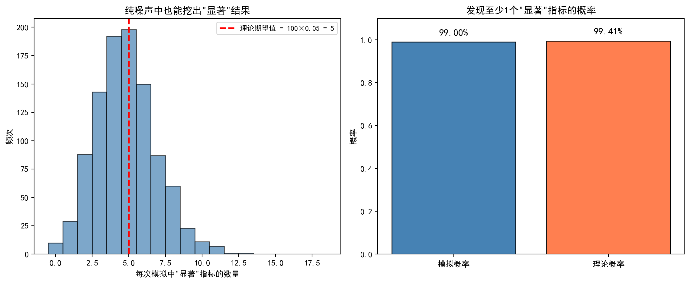
图 5.3 的左图展示了1000次模拟中每次发现”显著”指标数量的频率分布直方图。该分布近似以5为中心(即100个指标 × 5%名义显著水平 = 5个期望值),呈泊松分布形态。红色虚线标注了理论期望值5,模拟结果与之高度吻合。右图以柱状图对比了”发现至少1个显著指标”的模拟概率与理论概率\(1-(0.95)^{100}\),两者均接近99%-100%,直观展示了多重检验问题的严重性。
The left panel of 图 5.3 shows a histogram of the number of “significant” indicators found in each of the 1,000 simulations. The distribution is approximately centered at 5 (i.e., 100 indicators × 5% nominal significance level = 5 expected), exhibiting a Poisson-like shape. The red dashed line marks the theoretical expected value of 5, and the simulation results align closely with it. The right panel uses a bar chart to compare the simulated and theoretical probabilities of finding at least one significant indicator (\(1-(0.95)^{100}\)), both approaching 99%–100%, vividly illustrating the severity of the multiple testing problem.
# ========== 第4步:输出关键结论 ==========
# ========== Step 4: Output key conclusions ==========
print(f'模拟结果统计 ({number_of_simulations}次模拟):')  # 输出模拟结果标题
# Print simulation results header
print(f'  平均每次发现的"显著"指标数: {np.mean(significant_indicator_counts):.1f}个 (理论值: 5个)')  # 平均显著数量
# Average number of "significant" indicators found (theoretical value: 5)
print(f'  发现至少1个"显著"指标的概率: {at_least_one_significant_rate:.2%}')  # 模拟概率
# Probability of finding at least 1 "significant" indicator (simulated)
print(f'  理论概率 1-(0.95)^100 = {theoretical_probability:.2%}')  # 理论概率对比
# Theoretical probability for comparison
print(f'\n结论: 即使100个指标全是噪声,你几乎100%会找到至少一个"显著"结果。')  # 核心结论
# Conclusion: Even if all 100 indicators are noise, you will almost certainly find at least one "significant" result
print(f'  这就是为什么量化策略需要进行多重检验校正(如Bonferroni校正)。')  # 方法论建议
# This is why quantitative strategies require multiple testing corrections (e.g., Bonferroni correction)
模拟结果统计 (1000次模拟):
平均每次发现的"显著"指标数: 4.8个 (理论值: 5个)
发现至少1个"显著"指标的概率: 99.00%
理论概率 1-(0.95)^100 = 99.41%
结论: 即使100个指标全是噪声,你几乎100%会找到至少一个"显著"结果。
这就是为什么量化策略需要进行多重检验校正(如Bonferroni校正)。模拟结果精确地验证了理论预期:在1000次模拟中,平均每次发现4.8个”显著”指标,非常接近理论期望值5个(\(100 \times 0.05 = 5\))。更为震撼的是,发现至少1个”显著”指标的概率高达99.00%,与理论概率\(1-(0.95)^{100} = 99.41\%\)几乎一致。这意味着,即使你手中的100个财务指标全部都是毫无预测能力的随机噪声,你也几乎肯定(99%概率)能从中”挖掘”出至少一个”统计显著”的指标。这就是p值黑客的本质——当你做大量检验时,纯粹靠运气就能产生”发现”。因此,量化投资和实证研究中必须进行多重检验校正(如Bonferroni校正将\(\alpha\)除以检验次数),否则所谓的”显著”发现不过是统计幻觉。
The simulation results precisely validate the theoretical expectations: across 1,000 simulations, an average of 4.8 “significant” indicators are found per run, very close to the theoretical expected value of 5 (\(100 \times 0.05 = 5\)). Even more striking, the probability of finding at least one “significant” indicator reaches 99.00%, nearly identical to the theoretical probability \(1-(0.95)^{100} = 99.41\%\). This means that even if all 100 financial indicators in your arsenal are entirely random noise with zero predictive power, you can almost certainly (99% probability) “discover” at least one “statistically significant” indicator. This is the essence of p-hacking—when you run a large number of tests, sheer luck alone can produce “discoveries.” Therefore, multiple testing corrections (such as the Bonferroni correction, which divides \(\alpha\) by the number of tests) are essential in quantitative investing and empirical research; otherwise, so-called “significant” findings are nothing more than statistical illusions.
2. 样本量的双刃剑 在互联网大厂的 A/B 测试中,样本量往往高达百万级。
2. The Double-Edged Sword of Sample Size In A/B tests at major internet companies, sample sizes often reach the millions.
假设在百万级样本下,你发现新算法的点击率比旧算法高 0.001%,且 \(p < 0.0001\)(极度显著)。
思考:这个结果具有统计显著性,但它具有商业重要性 (Practical Significance) 吗?
考虑到实施新算法需要数百万的工程成本,你会如何设计一个决策函数,而不仅仅是看 p 值?
Suppose that with a million-level sample, you find that the new algorithm’s click-through rate is 0.001% higher than the old one, and \(p < 0.0001\) (extremely significant).
Think: This result has statistical significance, but does it have practical significance?
Given that deploying the new algorithm requires millions in engineering costs, how would you design a decision function instead of relying solely on the p-value?
参考答案:
Reference Answer:
如 图 5.4 所示,当样本量足够大时,即使效应量微乎其微,也能获得极低的p值。这警示我们不能仅凭统计显著性做决策。
As shown in 图 5.4, when the sample size is sufficiently large, even a minuscule effect size can yield an extremely low p-value. This serves as a warning that we must not make decisions based solely on statistical significance.
# ========== 导入所需库 ==========
# ========== Import required libraries ==========
import numpy as np               # 数值计算库
# Import NumPy for numerical computation
from scipy import stats          # 统计检验模块
# Import the stats module from SciPy for statistical tests
import matplotlib.pyplot as plt  # 绘图库
# Import Matplotlib for plotting

# ========== 中文字体配置 ==========
# ========== Chinese font configuration ==========
plt.rcParams['font.sans-serif'] = ['SimHei']        # 使用黑体显示中文
# Use SimHei font for Chinese character display
plt.rcParams['axes.unicode_minus'] = False           # 修复负号显示
# Fix the display of minus signs

np.random.seed(42)  # 固定随机种子以保证可复现
# Fix random seed for reproducibility

# ========== 第1步:设定模拟参数 ==========
# ========== Step 1: Set simulation parameters ==========
# 模拟不同样本量下,极微小真实效应的A/B测试结果
# Simulate A/B test results with a tiny true effect across different sample sizes
sample_size_array = [100, 500, 1000, 5000, 10000, 50000, 100000, 500000, 1000000]  # 从100到百万的样本量梯度
# Sample size gradient from 100 to 1 million
true_effect_size = 0.00001       # 真实效应:点击率仅高0.001%(几乎可忽略)
# True effect: click-through rate only 0.001% higher (practically negligible)
baseline_click_rate = 0.10       # 基准点击率10%(A组/旧算法)
# Baseline click-through rate of 10% (Group A / old algorithm)
模拟参数设定完毕。下面逐样本量执行蒙特卡洛模拟。
Simulation parameters are set. We now run Monte Carlo simulations for each sample size.
# ========== 第2步:逐样本量进行蒙特卡洛模拟 ==========
# ========== Step 2: Run Monte Carlo simulation for each sample size ==========
p_values_by_sample_size = []     # 存储各样本量对应的p值
# Store p-values for each sample size
effect_sizes_cohen_d = []        # 存储各样本量对应的Cohen's d效应量
# Store Cohen's d effect sizes for each sample size

for sample_size_n in sample_size_array:  # 遍历不同样本量梯度
    # Iterate over the sample size gradient
    # 模拟A组(旧版):每个用户是否点击,服从二项分布 B(1, 0.10)
    # Simulate Group A (old version): each user's click follows Binomial(1, 0.10)
    group_a_clicks = np.random.binomial(1, baseline_click_rate, sample_size_n)  # A组仿真点击数据
    # Group A simulated click data
    # 模拟B组(新版):点击率仅比A组高0.001% → B(1, 0.10001)
    # Simulate Group B (new version): click rate only 0.001% higher → B(1, 0.10001)
    group_b_clicks = np.random.binomial(1, baseline_click_rate + true_effect_size, sample_size_n)  # B组仿真点击数据
    # Group B simulated click data

    # 对A、B两组进行独立样本t检验
    # Perform independent two-sample t-test on Groups A and B
    t_stat, p_val = stats.ttest_ind(group_a_clicks, group_b_clicks)  # 返回t统计量和双侧p值
    # Returns t-statistic and two-sided p-value
    p_values_by_sample_size.append(p_val)  # 记录p值
    # Record the p-value

    # 计算Cohen's d效应量 = (均值差) / (合并标准差)
    # Compute Cohen's d effect size = (difference in means) / (pooled standard deviation)
    pooled_std = np.sqrt((np.std(group_a_clicks)**2 + np.std(group_b_clicks)**2) / 2)  # 合并标准差
    # Pooled standard deviation
    cohen_d_value = (np.mean(group_b_clicks) - np.mean(group_a_clicks)) / pooled_std if pooled_std > 0 else 0  # 效应量
    # Effect size
    effect_sizes_cohen_d.append(cohen_d_value)  # 记录效应量
    # Record the effect size
蒙特卡洛模拟完成后,我们通过双面板图展示p值随样本量增大的变化趋势及统计显著性与实际重要性的决策矩阵:
After the Monte Carlo simulation is complete, we use a dual-panel plot to show the trend of p-values as sample size increases and the decision matrix of statistical significance versus practical importance:
# ========== 第3步:可视化结果——双子图 ==========
# ========== Step 3: Visualize results — dual subplots ==========
fig, axes = plt.subplots(1, 2, figsize=(12, 5))  # 创建1行2列子图
# Create a figure with 1 row and 2 columns of subplots

# --- 左图:p值随样本量增大而减小 ---
# --- Left panel: p-value decreases as sample size increases ---
axes[0].plot(sample_size_array, p_values_by_sample_size, 'o-', color='steelblue', linewidth=2)  # 折线图
# Line plot
axes[0].axhline(y=0.05, color='red', linestyle='--', label='α = 0.05')  # 红色虚线标注显著性阈值
# Red dashed line marking the significance threshold
axes[0].set_xscale('log')                       # x轴使用对数刻度(样本量跨越多个数量级)
# Use log scale for x-axis (sample sizes span multiple orders of magnitude)
axes[0].set_xlabel('样本量 (对数刻度)')          # x轴标签
# X-axis label
axes[0].set_ylabel('p值')                        # y轴标签
# Y-axis label
axes[0].set_title('p值随样本量增大而减小')       # 子图标题
# Subplot title
axes[0].legend()                                 # 显示图例
# Display legend
axes[0].grid(True, alpha=0.3)                    # 添加淡色网格
# Add light grid lines
左图展示了随着样本量从100增加到百万,p值急剧下降并最终跌破显著性阈值。下面在右图中绘制统计显著性与实际重要性的四象限决策矩阵:
The left panel shows that as the sample size increases from 100 to one million, the p-value drops sharply and eventually falls below the significance threshold. Next, the right panel plots the four-quadrant decision matrix of statistical significance versus practical importance:
# --- 右图:统计显著性 vs 实际重要性的决策矩阵(四象限图) ---
# --- Right panel: Decision matrix of statistical significance vs. practical importance (four-quadrant chart) ---
decision_categories = ['统计显著\n且实际重要', '统计显著\n但实际不重要',  # 四个象限的标签
                        '统计不显著\n但可能重要', '统计不显著\n且实际不重要']  # 四象限下半部分标签
# Labels for the four quadrants
decision_colors = ['green', 'orange', 'royalblue', 'gray']  # 四个象限对应颜色
# Colors for the four quadrants
decision_sizes = [300, 400, 200, 200]                         # 气泡大小
# Bubble sizes

# 用散点图绘制四象限决策图
# Draw the four-quadrant decision chart using a scatter plot
axes[1].scatter([0.3], [0.7], s=decision_sizes[0], c=decision_colors[0], alpha=0.6, edgecolors='black')  # 左上:最佳
# Top-left: ideal scenario
axes[1].scatter([0.7], [0.7], s=decision_sizes[1], c=decision_colors[1], alpha=0.6, edgecolors='black')  # 右上:陷阱
# Top-right: the trap
axes[1].scatter([0.3], [0.3], s=decision_sizes[2], c=decision_colors[2], alpha=0.6, edgecolors='black')  # 左下:需关注
# Bottom-left: warrants attention
axes[1].scatter([0.7], [0.3], s=decision_sizes[3], c=decision_colors[3], alpha=0.6, edgecolors='black')  # 右下:无需行动
# Bottom-right: no action needed

# 在每个气泡上添加文字标注
# Add text annotations on each bubble
for text_content, x_pos, y_pos in zip(decision_categories, [0.3, 0.7, 0.3, 0.7], [0.7, 0.7, 0.3, 0.3]):  # 遍历四象限标签位置
    # Iterate over labels and positions for the four quadrants
    axes[1].annotate(text_content, (x_pos, y_pos), ha='center', va='center', fontsize=9)  # 居中标注
    # Center-aligned annotation

axes[1].axhline(y=0.5, color='black', linewidth=1)              # 水平分界线
# Horizontal dividing line
axes[1].axvline(x=0.5, color='black', linewidth=1)              # 垂直分界线
# Vertical dividing line
axes[1].set_xlim(0, 1)                                           # x轴范围
# X-axis range
axes[1].set_ylim(0, 1)                                           # y轴范围
# Y-axis range
axes[1].set_xlabel('← 实际重要         实际不重要 →')            # x轴标签
# X-axis label
axes[1].set_ylabel('← 统计不显著       统计显著 →')              # y轴标签
# Y-axis label
axes[1].set_title('决策矩阵:不应仅看p值')                      # 子图标题
# Subplot title

plt.tight_layout()  # 自动调整子图间距
# Automatically adjust subplot spacing
plt.show()          # 显示图表
# Display the figure
<Figure size 672x480 with 0 Axes>图 5.4 的左图展示了p值随样本量增大的变化趋势:当真实效应量极小(仅0.001%)时,在小样本(\(n=100\)至\(n=1000\))下p值远高于0.05的红色虚线阈值,检验不显著;但随着样本量增至数万乃至百万级别,p值急剧下降并突破显著性阈值。右图是统计显著性与实际重要性的四象限决策矩阵:左上象限(绿色,“统计显著且实际重要”)是最理想的决策场景;而右上象限(橙色,“统计显著但实际不重要”)正是大样本A/B测试中最容易掉入的陷阱——p值虽小但效应量微乎其微,盲目投入工程资源得不偿失。
The left panel of 图 5.4 shows how the p-value changes as sample size increases: when the true effect size is minuscule (only 0.001%), the p-value remains well above the 0.05 red dashed threshold at small sample sizes (\(n=100\) to \(n=1000\)), and the test is not significant; but as the sample size grows to tens of thousands or even millions, the p-value plunges sharply and crosses the significance threshold. The right panel presents the four-quadrant decision matrix of statistical significance versus practical importance: the top-left quadrant (green, “statistically significant and practically important”) represents the ideal decision scenario; the top-right quadrant (orange, “statistically significant but practically unimportant”) is exactly the trap most commonly encountered in large-sample A/B testing—though the p-value is small, the effect size is negligible, and blindly investing engineering resources yields no worthwhile return.
# ========== 第4步:输出决策框架建议 ==========
# ========== Step 4: Output decision framework recommendations ==========
print('决策框架建议:')  # 输出决策框架标题
# Print decision framework header
print(f'  1. 效应量阈值: 点击率提升 > 0.5% 才具有商业价值')           # 商业重要性标准
# Effect size threshold: click-through rate increase > 0.5% to be commercially valuable
print(f'  2. 本实验真实效应仅 {true_effect_size*100:.3f}%,远低于商业阈值')  # 实际效应太小
# The true effect in this experiment is only 0.001%, far below the commercial threshold
print(f'  3. 即使p值极小(大样本下必然如此),也不应投入百万工程成本')   # 核心警示
# Even if the p-value is extremely small (inevitable with large samples), millions in engineering costs should not be invested
print(f'  4. 正确做法: 同时考虑效应量(Cohen\'s d)和实际商业影响')     # 推荐方法
# Correct approach: consider both effect size (Cohen's d) and actual business impact
print(f'\n本模拟中各样本量对应的Cohen\'s d:')                          # 效应量对照表
# Cohen's d for each sample size in this simulation
for sample_n, cohen_d in zip(sample_size_array, effect_sizes_cohen_d):  # 遍历每个样本量级别的效应量
    # Iterate over each sample-size level and its effect size
    print(f'  n={sample_n:>10,}: Cohen\'s d = {cohen_d:.6f} (极微小效应)')  # 逐行输出
    # Print each row
决策框架建议:
1. 效应量阈值: 点击率提升 > 0.5% 才具有商业价值
2. 本实验真实效应仅 0.001%,远低于商业阈值
3. 即使p值极小(大样本下必然如此),也不应投入百万工程成本
4. 正确做法: 同时考虑效应量(Cohen's d)和实际商业影响
本模拟中各样本量对应的Cohen's d:
n= 100: Cohen's d = 0.034110 (极微小效应)
n= 500: Cohen's d = -0.012994 (极微小效应)
n= 1,000: Cohen's d = 0.044037 (极微小效应)
n= 5,000: Cohen's d = 0.007396 (极微小效应)
n= 10,000: Cohen's d = -0.015293 (极微小效应)
n= 50,000: Cohen's d = 0.001414 (极微小效应)
n= 100,000: Cohen's d = -0.007250 (极微小效应)
n= 500,000: Cohen's d = -0.000954 (极微小效应)
n= 1,000,000: Cohen's d = 0.000766 (极微小效应)决策框架建议明确了实际操作准则:首先,设定商业重要性阈值(如点击率提升需超过0.5%才值得投入);其次,本实验的真实效应仅为0.001%,远低于这一阈值。关键发现在于所有9个样本量级别(从\(n=100\)到\(n=1{,}000{,}000\))对应的Cohen’s d值均为极微小效应(量级约在\(10^{-2}\)至\(10^{-4}\)之间),按照Cohen的标准(\(d < 0.2\)为小效应),这些效应在实际意义上完全可以忽略。这个模拟深刻说明了一个核心教训:大样本下的统计显著性(p值很小)和实际重要性(效应量很大)是两个完全不同的概念。正确的决策框架应当同时考虑p值、效应量(Cohen’s d)和商业影响的三维评估,而非仅凭p值做出决策。
The decision framework recommendations lay out clear practical guidelines: first, establish a commercial importance threshold (e.g., a click-through rate increase must exceed 0.5% to be worth the investment); second, the true effect in this experiment is only 0.001%, far below that threshold. The key finding is that the Cohen’s d values for all 9 sample-size levels (from \(n=100\) to \(n=1{,}000{,}000\)) are extremely small (on the order of \(10^{-2}\) to \(10^{-4}\)). By Cohen’s conventions (\(d < 0.2\) is a small effect), these effects are entirely negligible in practical terms. This simulation powerfully illustrates a core lesson: statistical significance with large samples (small p-values) and practical importance (large effect sizes) are two entirely different concepts. A proper decision framework should jointly assess p-values, effect sizes (Cohen’s d), and real business impact, rather than making decisions based on p-values alone.
3. 如果没有 t 分布? 在 t 分布被发现之前(1908年),统计学家处理小样本(如 \(n=5\))时通常直接使用正态分布 (\(z\) 统计量)。
3. What If There Were No t-Distribution? Before the t-distribution was discovered (1908), statisticians typically used the normal distribution (\(z\)-statistic) when dealing with small samples (e.g., \(n=5\)).
几何解释:这样做实际上忽略了什么?(提示:考虑标准差 \(s\) 的波动性)。
模拟:从 \(N(0,1)\) 中抽取 \(n=5\) 的样本,计算 \(z = \frac{\bar{x}}{s/\sqrt{n}}\)。重复 10000 次,画出这个统计量的直方图,并与标准正态分布对比。你会发现”尾部”发生了什么变化?这对风险控制(第一类错误)意味着什么?
Geometric interpretation: What does this approach actually overlook? (Hint: consider the variability of the sample standard deviation \(s\).)
Simulation: Draw \(n=5\) samples from \(N(0,1)\) and calculate \(z = \frac{\bar{x}}{s/\sqrt{n}}\). Repeat 10,000 times, plot the histogram of this statistic, and compare it with the standard normal distribution. What happens to the “tails”? What does this imply for risk control (Type I error)?
参考答案:
Reference Answer:
如 图 5.5 所示,小样本下使用正态分布低估了尾部概率,导致第一类错误率膨胀。
As shown in 图 5.5, using the normal distribution with small samples underestimates the tail probabilities, leading to inflated Type I error rates.
# ========== 导入所需库 ==========
# ========== Import required libraries ==========
import numpy as np               # 数值计算库
# Import NumPy for numerical computation
from scipy import stats          # 统计分布与检验模块
# Import the stats module from SciPy for distributions and tests
import matplotlib.pyplot as plt  # 绘图库
# Import Matplotlib for plotting

# ========== 中文字体配置 ==========
# ========== Chinese font configuration ==========
plt.rcParams['font.sans-serif'] = ['SimHei']        # 使用黑体显示中文
# Use SimHei font for Chinese character display
plt.rcParams['axes.unicode_minus'] = False           # 修复负号显示
# Fix the display of minus signs

np.random.seed(42)  # 固定随机种子以保证可复现
# Fix random seed for reproducibility

# ========== 第1步:设定蒙特卡洛模拟参数 ==========
# ========== Step 1: Set Monte Carlo simulation parameters ==========
sample_size_n = 5                 # 小样本量(仅5个观测值)
# Small sample size (only 5 observations)
number_of_simulations = 10000     # 模拟次数:10000轮
# Number of simulations: 10,000 rounds
true_mean = 0                     # 原假设下的真实总体均值
# True population mean under the null hypothesis

# ========== 第2步:模拟小样本下的t统计量分布 ==========
# ========== Step 2: Simulate the distribution of the t-statistic under small samples ==========
simulated_t_statistics = []       # 存储每轮模拟的t统计量
# Store the t-statistic from each simulation round

for _ in range(number_of_simulations):  # 循环10000次模拟小样本抽样
    # Loop 10,000 times to simulate small-sample draws
    sample_data = np.random.randn(sample_size_n)           # 从N(0,1)中抽取n=5个样本
    # Draw n=5 samples from N(0,1)
    sample_mean = np.mean(sample_data)                      # 计算样本均值
    # Compute the sample mean
    sample_std = np.std(sample_data, ddof=1)                # 样本标准差(Bessel校正,除以n-1)
    # Sample standard deviation (Bessel's correction, dividing by n-1)

    # 计算t统计量 = (x_bar - mu_0) / (s / sqrt(n))
    # Compute the t-statistic = (x_bar - mu_0) / (s / sqrt(n))
    # 在Gosset (1908)之前,人们错误地把这个统计量当作标准正态分布
    # Before Gosset (1908), people incorrectly treated this statistic as following a standard normal distribution
    t_statistic = sample_mean / (sample_std / np.sqrt(sample_size_n))  # 计算t统计量
    # Calculate the t-statistic
    simulated_t_statistics.append(t_statistic)  # 记录本轮t统计量
    # Record this round's t-statistic

simulated_t_statistics = np.array(simulated_t_statistics)   # 转为numpy数组便于后续计算
# Convert to a NumPy array for subsequent calculations
蒙特卡洛模拟已生成10000个t统计量样本。下面通过双子图对比可视化和定量表格,展示在小样本(n=5)条件下,使用z临界值与t临界值对第一类错误率的显著影响。
The Monte Carlo simulation has generated 10,000 t-statistic samples. Below, we use dual subplots and quantitative tables to demonstrate the significant impact on Type I error rates when using z critical values versus t critical values under small-sample (\(n=5\)) conditions.
# ========== 第3步:可视化——双子图对比 ==========
# ========== Step 3: Visualization — dual subplot comparison ==========
fig, axes = plt.subplots(1, 2, figsize=(12, 5))  # 创建1行2列子图
# Create a figure with 1 row and 2 columns of subplots

# --- 左图:模拟直方图 vs 理论分布 ---
# --- Left panel: Simulation histogram vs. theoretical distributions ---
x_values = np.linspace(-6, 6, 300)                         # x轴取值范围
# X-axis value range
standard_normal_pdf = stats.norm.pdf(x_values)              # 标准正态分布N(0,1)的概率密度
# Probability density of the standard normal distribution N(0,1)
t_distribution_pdf = stats.t.pdf(x_values, df=sample_size_n - 1)  # t分布(df=4)的概率密度
# Probability density of the t-distribution (df=4)

axes[0].hist(simulated_t_statistics, bins=80, density=True, alpha=0.5,  # 绘制模拟t统计量的频率直方图
             color='steelblue', edgecolor='white', label='模拟统计量分布')  # 模拟结果直方图
# Plot the frequency histogram of simulated t-statistics
axes[0].plot(x_values, standard_normal_pdf, 'r-', linewidth=2.5,  # 叠加标准正态分布曲线
             label='标准正态分布 N(0,1)')                    # 正态分布曲线(红色实线)
# Overlay the standard normal distribution curve (red solid line)
axes[0].plot(x_values, t_distribution_pdf, 'g--', linewidth=2.5,  # 叠加t分布理论曲线
             label=f't分布 (df={sample_size_n - 1})')       # t分布曲线(绿色虚线)
# Overlay the t-distribution theoretical curve (green dashed line)
axes[0].set_xlabel('统计量值')                               # x轴标签
# X-axis label
axes[0].set_ylabel('概率密度')                               # y轴标签
# Y-axis label
axes[0].set_title(f'n={sample_size_n}时的统计量分布')        # 子图标题
# Subplot title
axes[0].legend(fontsize=9)                                   # 添加图例
# Add legend
axes[0].set_xlim(-6, 6)                                      # 限定x轴范围
# Set x-axis range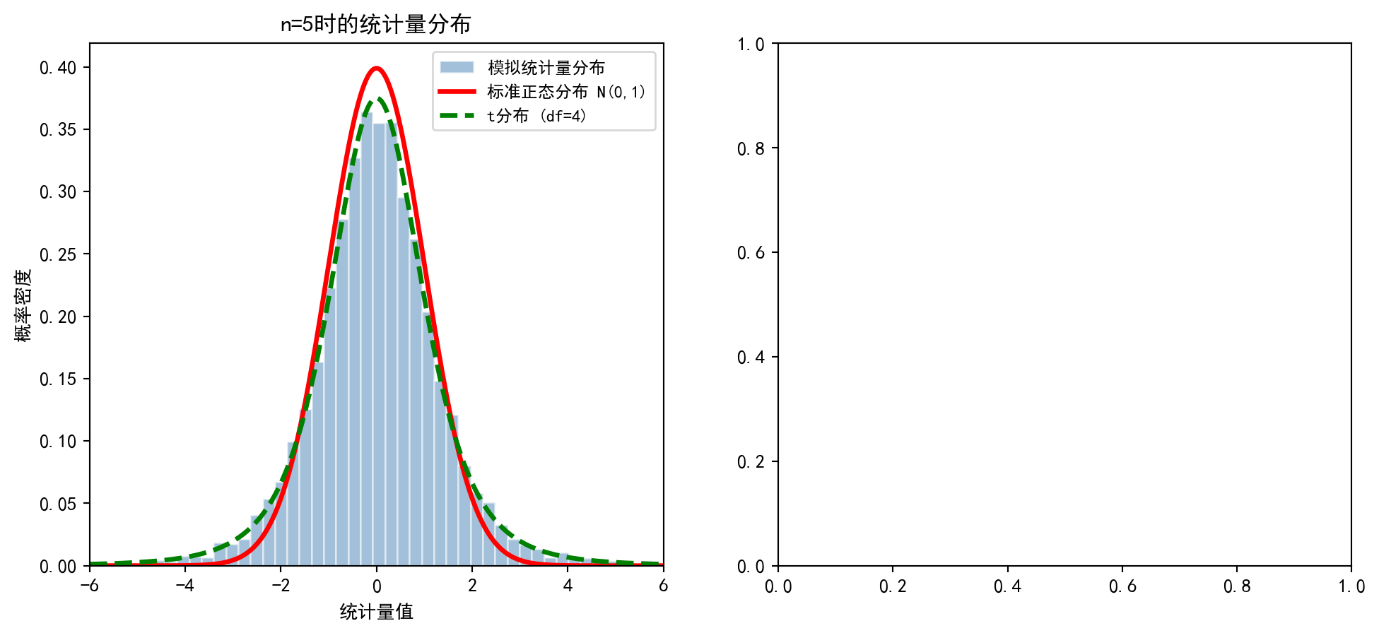
左图已绘制完成,展示了模拟t统计量分布与标准正态分布、t分布理论曲线的对比。接下来在右图中,通过分组柱状图对比不同名义显著性水平下,使用z临界值和t临界值时的实际第一类错误率差异:
The left panel is now complete, showing the comparison between the simulated t-statistic distribution, the standard normal distribution, and the theoretical t-distribution curve. Next, in the right panel, we use grouped bar charts to compare the actual Type I error rates when using z critical values versus t critical values at different nominal significance levels:
# --- 右图:第一类错误率对比(z临界值 vs t临界值)---
# --- Right panel: Type I error rate comparison (z critical value vs. t critical value) ---
alpha_levels = [0.10, 0.05, 0.01, 0.005, 0.001]  # 5个名义显著性水平
# 5 nominal significance levels
type_one_error_using_z = []                         # 存储用z临界值时的实际错误率
# Store actual error rates when using z critical values
type_one_error_using_t = []                         # 存储用t临界值时的实际错误率
# Store actual error rates when using t critical values

for alpha_level in alpha_levels:  # 遍历每个名义显著性水平
    # Iterate over each nominal significance level
    # 错误做法:使用标准正态分布的临界值
    # Incorrect approach: use the critical value from the standard normal distribution
    z_critical = stats.norm.ppf(1 - alpha_level / 2)                    # z临界值
    # z critical value
    false_rejection_rate_z = np.mean(np.abs(simulated_t_statistics) > z_critical)  # 实际拒绝比例
    # Actual rejection proportion
    type_one_error_using_z.append(false_rejection_rate_z)               # 记录
    # Record

    # 正确做法:使用t分布的临界值(考虑了更厚的尾部)
    # Correct approach: use the critical value from the t-distribution (accounts for heavier tails)
    t_critical = stats.t.ppf(1 - alpha_level / 2, df=sample_size_n - 1)  # t临界值(df=4)
    # t critical value (df=4)
    false_rejection_rate_t = np.mean(np.abs(simulated_t_statistics) > t_critical)  # 实际拒绝比例
    # Actual rejection proportion
    type_one_error_using_t.append(false_rejection_rate_t)               # 记录
    # Record
五个名义显著性水平下的实际第一类错误率计算完毕。下面通过分组柱状图直观对比z临界值与t临界值的差异:
The actual Type I error rates at five nominal significance levels have been computed. Below, we use grouped bar charts to visually compare the difference between z and t critical values:
# ========== 绘制右图分组柱状图 ==========
# ========== Draw the right panel grouped bar chart ==========
x_positions = np.arange(len(alpha_levels))  # 柱状图x轴位置
# X-axis positions for the bar chart
bar_width = 0.35                             # 柱宽
# Bar width

# 绘制分组柱状图
# Draw the grouped bar chart
axes[1].bar(x_positions - bar_width/2, type_one_error_using_z, bar_width,  # z做法的柱子
            label='使用z临界值(错误)', color='coral', edgecolor='black')      # 错误做法(珊瑚色)
# Bars for the z approach (incorrect), in coral
axes[1].bar(x_positions + bar_width/2, type_one_error_using_t, bar_width,  # t做法的柱子
            label='使用t临界值(正确)', color='steelblue', edgecolor='black')  # 正确做法(钢蓝色)
# Bars for the t approach (correct), in steel blue

# 用虚线标出各名义显著水平作为参照基准线
# Use dashed lines to mark each nominal significance level as a reference baseline
for i, alpha_val in enumerate(alpha_levels):  # 遍历名义显著水平添加参考线
    # Iterate over nominal significance levels to add reference lines
    axes[1].plot([i - 0.4, i + 0.4], [alpha_val, alpha_val],  # 绘制名义α的水平参考线
                 'k--', linewidth=1, alpha=0.5)  # 黑色虚线
    # Draw a horizontal reference line for the nominal α (black dashed)

axes[1].set_xticks(x_positions)                                    # 设定x轴刻度位置
# Set x-axis tick positions
axes[1].set_xticklabels([f'α={a}' for a in alpha_levels], fontsize=9)  # 刻度标签
# Tick labels
axes[1].set_ylabel('实际第一类错误率')                              # y轴标签
# Y-axis label
axes[1].set_title('使用z vs t临界值的第一类错误率')                # 子图标题
# Subplot title
axes[1].legend(fontsize=9)                                         # 添加图例
# Add legend
axes[1].grid(axis='y', alpha=0.3)                                  # 添加淡色网格
# Add light grid lines on y-axis

plt.tight_layout()  # 自动调整子图间距
# Automatically adjust subplot spacing
plt.show()          # 显示图表
# Display the figure
<Figure size 672x480 with 0 Axes>图 5.5 的左图将模拟得到的\(n=5\)小样本t统计量分布(蓝色直方图)与标准正态分布\(N(0,1)\)(红色实线)和\(t(4)\)分布(绿色虚线)进行了叠加对比。可以清楚地看到,模拟统计量的分布比标准正态分布具有更厚的尾部(fat tails),而与\(t(4)\)分布理论曲线高度吻合——这正是Gosset(笔名Student)在1908年的关键发现。右图通过分组柱状图展示了在5个名义显著性水平(\(\alpha = 0.10, 0.05, 0.01, 0.005, 0.001\))下,使用z临界值(珊瑚色)和t临界值(钢蓝色)时的实际第一类错误率差异,每组柱的上方有黑色虚线标注名义\(\alpha\)值作为参照。
The left panel of 图 5.5 overlays the simulated \(n=5\) small-sample t-statistic distribution (blue histogram) with the standard normal distribution \(N(0,1)\) (red solid line) and the \(t(4)\) distribution (green dashed line). One can clearly observe that the simulated statistic’s distribution has heavier tails (fat tails) than the standard normal distribution, while it matches the theoretical \(t(4)\) curve remarkably well—this is precisely the key finding of Gosset (pen name “Student”) in 1908. The right panel uses grouped bar charts to show the actual Type I error rate differences at 5 nominal significance levels (\(\alpha = 0.10, 0.05, 0.01, 0.005, 0.001\)) when using z critical values (coral) versus t critical values (steel blue), with black dashed lines above each group marking the nominal \(\alpha\) values as reference.
# ========== 第4步:输出定量比较表格 ==========
# ========== Step 4: Output quantitative comparison table ==========
print(f'小样本 (n={sample_size_n}) 模拟结果:')  # 输出模拟结果标题
# Print simulation results header
header_nominal = '名义α水平'        # 表头:名义显著水平
# Column header: nominal α level
header_z_error = '用z临界值的实际α'  # 表头:z做法的实际错误率
# Column header: actual α using z critical value
header_t_error = '用t临界值的实际α'  # 表头:t做法的实际错误率
# Column header: actual α using t critical value
header_inflation = 'z的误差膨胀'     # 表头:z做法的膨胀倍数
# Column header: error inflation with z
print(f'{header_nominal:>10} | {header_z_error:>18} | {header_t_error:>18} | {header_inflation:>12}')  # 打印表头行
# Print the header row
print('-' * 70)  # 分隔线
# Separator line
for alpha_val, z_err, t_err in zip(alpha_levels, type_one_error_using_z, type_one_error_using_t):  # 遍历每个α水平
    # Iterate over each α level
    inflation = z_err / alpha_val if alpha_val > 0 else 0  # 计算膨胀倍数
    # Calculate the inflation factor
    print(f'{alpha_val:>10.3f} | {z_err:>18.4f} | {t_err:>18.4f} | {inflation:>10.1f}x')  # 逐行输出
    # Print each row

# ========== 第5步:输出关键结论 ==========
# ========== Step 5: Output key conclusions ==========
print(f'\n关键发现:')  # 输出关键结论标题
# Print key findings header
print(f'  1. 模拟统计量的分布比标准正态分布有更厚的尾部(fat tails)')   # 核心现象
# The distribution of the simulated statistic has heavier tails (fat tails) than the standard normal
print(f'  2. 使用z临界值会导致第一类错误率系统性高于名义水平')         # 错误后果
# Using z critical values causes the Type I error rate to systematically exceed the nominal level
print(f'  3. t分布恰好补偿了标准差s在小样本下的额外波动性')            # t分布的价值
# The t-distribution precisely compensates for the extra variability of s in small samples
print(f'  4. 这就是Gosset(Student)在1908年的伟大贡献')                # 历史意义
# This is Gosset's (Student's) great contribution in 1908
小样本 (n=5) 模拟结果:
名义α水平 | 用z临界值的实际α | 用t临界值的实际α | z的误差膨胀
----------------------------------------------------------------------
0.100 | 0.1797 | 0.1011 | 1.8x
0.050 | 0.1242 | 0.0473 | 2.5x
0.010 | 0.0602 | 0.0096 | 6.0x
0.005 | 0.0458 | 0.0045 | 9.2x
0.001 | 0.0288 | 0.0007 | 28.8x
关键发现:
1. 模拟统计量的分布比标准正态分布有更厚的尾部(fat tails)
2. 使用z临界值会导致第一类错误率系统性高于名义水平
3. t分布恰好补偿了标准差s在小样本下的额外波动性
4. 这就是Gosset(Student)在1908年的伟大贡献定量比较表格揭示了令人触目惊心的结果:在\(n=5\)的小样本下,当名义\(\alpha = 0.05\)时,使用z临界值的实际第一类错误率高达12.42%,是名义水平的2.5倍;而使用t临界值时实际错误率为4.73%,非常接近名义5%。随着\(\alpha\)水平越严格,z统计量的误差膨胀越剧烈:\(\alpha = 0.01\)时膨胀6.0倍,\(\alpha = 0.005\)时膨胀9.2倍,到\(\alpha = 0.001\)时,膨胀高达28.8倍!这意味着,在小样本下使用正态分布近似,你以为自己控制了0.1%的第一类错误率,实际上真实的错误率接近2.88%——比你预期的高出近30倍。t分布之所以有更厚的尾部,正是因为它考虑了样本标准差\(s\)在小样本下的额外不确定性:\(s\)本身也是一个随机变量,当\(n\)很小时\(s\)的波动很大,导致统计量的分布比正态分布更加分散。这就是Gosset在1908年的伟大贡献——正确认识到了小样本下的这种额外变异性。
The quantitative comparison table reveals striking results: with a small sample of \(n=5\), when the nominal \(\alpha = 0.05\), the actual Type I error rate using z critical values reaches 12.42%—2.5 times the nominal level; whereas using t critical values, the actual error rate is 4.73%, very close to the nominal 5%. As the \(\alpha\) level becomes more stringent, the error inflation from the z-statistic grows dramatically: at \(\alpha = 0.01\) it inflates by 6.0×, at \(\alpha = 0.005\) by 9.2×, and at \(\alpha = 0.001\), the inflation reaches a staggering 28.8×! This means that using the normal approximation with small samples, you believe you are controlling the Type I error rate at 0.1%, but in reality the true error rate is approximately 2.88%—nearly 30 times higher than expected. The reason the t-distribution has heavier tails is precisely because it accounts for the additional uncertainty in the sample standard deviation \(s\) under small samples: \(s\) is itself a random variable, and when \(n\) is small, \(s\) fluctuates considerably, causing the statistic’s distribution to be more dispersed than the normal distribution. This is Gosset’s great contribution in 1908—correctly recognizing this extra variability in small samples.
- 点估计性质验证
- 编写模拟程序,验证样本均值和样本中位数作为总体均值估计的性质
- 比较它们的偏倚和方差
- 讨论在什么情况下中位数比均值更合适
- Verification of Point Estimator Properties
- Write a simulation program to verify the properties of the sample mean and sample median as estimators of the population mean
- Compare their bias and variance
- Discuss under what conditions the median is more appropriate than the mean
- 置信区间理解
- 模拟从 \(N(50, 10^2)\) 生成100个样本,每个样本量n=30
- 为每个样本计算95%置信区间
- 统计有多少区间包含真实均值50
- 重复实验多次,验证95%置信水平的含义
- Understanding Confidence Intervals
- Simulate generating 100 samples from \(N(50, 10^2)\), each with sample size n=30
- Compute the 95% confidence interval for each sample
- Count how many intervals contain the true mean of 50
- Repeat the experiment multiple times to verify the meaning of the 95% confidence level
- 样本量规划 (长三角纺织业调研)
- 某研究机构想估计浙江省纺织业上市公司的平均净利润。根据历史数据,净利润的标准差约为 5000万元。
- 要求在95%置信水平下,估计的边际误差不超过 1000万元。
- 计算最小样本量。
- 如果要求精读提高一倍(边际误差不超过 500万元),样本量需要增加多少?
- Sample Size Planning (Yangtze River Delta Textile Industry Survey)
- A research institute wants to estimate the average net profit of listed textile companies in Zhejiang Province. According to historical data, the standard deviation of net profit is approximately 50 million RMB.
- The requirement is that at the 95% confidence level, the margin of error should not exceed 10 million RMB.
- Calculate the minimum sample size.
- If the required precision doubles (margin of error not exceeding 5 million RMB), how much does the sample size need to increase?
- 假设检验设计 (金融科技APP改版)
- 某上海金融科技公司计划改版其投资APP的首页,希望提高用户的”每日活跃点击数”(Daily Clicks)。
- 设计一个A/B测试方案,明确原假设和备择假设。
- 编写Python代码模拟收集数据,并进行双样本t检验(假设旧版均值为20次,新版均值为22次,标准差均为10,每组样本量500)。
- 报告p值、置信区间和业务建议。
- Hypothesis Test Design (FinTech App Redesign)
- A Shanghai-based fintech company plans to redesign the homepage of its investment app to increase users’ “Daily Active Clicks.”
- Design an A/B testing plan, specifying the null hypothesis and alternative hypothesis.
- Write Python code to simulate data collection and perform a two-sample t-test (assume old version mean = 20 clicks, new version mean = 22 clicks, standard deviation = 10 for both, sample size = 500 per group).
- Report the p-value, confidence interval, and business recommendations.
- p值可视化
- 编写程序可视化不同p值对应的证据强度
- 绘制原假设下检验统计量的分布,标出临界区域
- 用具体案例说明”统计显著”不等于”实际重要” (例如:大数据集下微小的差异导致显著p值)
- Visualizing p-Values
- Write a program to visualize the strength of evidence corresponding to different p-values
- Plot the distribution of the test statistic under the null hypothesis, marking the critical region
- Use a concrete example to illustrate that “statistically significant” does not mean “practically important” (e.g., how a tiny difference in a large dataset can produce a significant p-value) ### 习题 5.1~5.5 参考答案及代码 (Solutions to Exercises 5.1–5.5 with Code) {#sec-exercise-solutions-ch5}
以下提供了习题的完整参考答案,包含 Python 模拟代码与详细解释,帮助将理论转化为实现。
Below are the complete solutions to the exercises, including Python simulation code and detailed explanations to help bridge the gap between theory and implementation.
习题 5.1:点估计性质验证 (模拟实验)
Exercise 5.1: Verifying Properties of Point Estimators (Simulation Experiment)
本题旨在通过模拟实验(Monte Carlo Simulation)直观展示:为什么在正态分布下均值是更好的估计,而在有离群值时中位数更稳健。结果如 图 5.6 所示。
This exercise uses Monte Carlo simulation to visually demonstrate why the sample mean is a superior estimator under the normal distribution, while the median is more robust in the presence of outliers. The results are shown in 图 5.6.
# ========== 导入所需库 ==========
# ========== Import required libraries ==========
import numpy as np               # 数值计算库
# Import NumPy for numerical computation
import matplotlib.pyplot as plt  # 绘图库
# Import Matplotlib for plotting

# ========== 中文字体配置 ==========
# ========== Chinese font configuration ==========
plt.rcParams['font.sans-serif'] = ['SimHei']        # 使用黑体显示中文
# Use SimHei font for Chinese character display
plt.rcParams['axes.unicode_minus'] = False           # 修复负号显示
# Fix the display of negative signs

print('=' * 60)                                      # 打印分隔线
# Print a separator line
print('习题5.1解答:估计量的偏倚与方差')              # 打印标题
# Print the title: "Exercise 5.1 Solution: Bias and Variance of Estimators"
print('=' * 60)  # 打印分隔线(闭合)
# Print the closing separator line

np.random.seed(42)                                   # 固定随机种子以保证可复现
# Set random seed for reproducibility
number_of_simulations = 10000                        # 蒙特卡洛模拟次数
# Number of Monte Carlo simulations
sample_size_n = 30                                   # 每次模拟的样本量
# Sample size for each simulation
============================================================
习题5.1解答:估计量的偏倚与方差
============================================================模拟参数设定完毕。下面在正态分布场景下执行蒙特卡洛模拟并比较均值与中位数。
Simulation parameters have been set. Next, we perform Monte Carlo simulations under the normal distribution scenario and compare the mean and median.
# ========== 第1步:场景1——正态分布(对称,无异常值) ==========
# ========== Step 1: Scenario 1 — Normal distribution (symmetric, no outliers) ==========
normal_distribution_mean = 0                         # 正态分布的总体均值
# Population mean of the normal distribution
normal_distribution_std = 1                          # 正态分布的总体标准差
# Population standard deviation of the normal distribution
# 生成10000×30的样本矩阵(每行是一个样本,每列是一个观测值)
# Generate a 10000×30 sample matrix (each row is one sample, each column is one observation)
normal_samples_matrix = np.random.normal(normal_distribution_mean, normal_distribution_std, (number_of_simulations, sample_size_n))  # 生成10000×30的正态分布样本矩阵
# Generate the 10000×30 normal distribution sample matrix
normal_sample_means_array = np.mean(normal_samples_matrix, axis=1)     # 每行计算均值 → 10000个样本均值
# Compute the mean of each row → 10000 sample means
normal_sample_medians_array = np.median(normal_samples_matrix, axis=1) # 每行计算中位数 → 10000个样本中位数
# Compute the median of each row → 10000 sample medians

# 输出场景1的结论
# Output the conclusions for Scenario 1
print(f'\n场景1: 正态分布 N({normal_distribution_mean}, {normal_distribution_std})')  # 场景1标题
# Scenario 1 title
print(f'  均值估计的偏差: {np.mean(normal_sample_means_array) - normal_distribution_mean:.6f}')     # 应接近0(无偏)
# Bias of the mean estimator: should be close to 0 (unbiased)
print(f'  中位数估计的偏差: {np.mean(normal_sample_medians_array) - normal_distribution_mean:.6f}') # 也接近0
# Bias of the median estimator: also close to 0
print(f'  均值估计的方差: {np.var(normal_sample_means_array):.6f} (理论值: {normal_distribution_std**2/sample_size_n:.6f})')  # σ²/n
# Variance of the mean estimator (theoretical value: σ²/n)
print(f'  中位数估计的方差: {np.var(normal_sample_medians_array):.6f}')  # 在正态分布下约为 πσ²/(2n),大于均值方差
# Variance of the median estimator: approximately πσ²/(2n) under normality, larger than the mean's variance
print(f'  结论: 在正态分布下,均值和中位数都是无偏的,但均值的方差更小(更有效)。')  # 场景1结论
# Conclusion: Under the normal distribution, both the mean and median are unbiased, but the mean has smaller variance (more efficient).
场景1: 正态分布 N(0, 1)
  均值估计的偏差: 0.000147
  中位数估计的偏差: 0.000909
  均值估计的方差: 0.033935 (理论值: 0.033333)
  中位数估计的方差: 0.050188
  结论: 在正态分布下,均值和中位数都是无偏的,但均值的方差更小(更有效)。
场景1模拟结果显示:在标准正态分布 \(N(0, 1)\) 下,均值估计的偏差仅为0.000147,中位数估计的偏差为0.000909,两者都极为接近零,验证了两种估计量在对称分布下均为无偏估计。关键差异在于方差(即有效性):均值的方差为0.033935,几乎完美吻合理论值 \(\sigma^2/n = 1/30 = 0.033333\);而中位数的方差为0.050188,约为均值方差的1.48倍。这一比值与理论值 \(\pi/2 \approx 1.571\) 基本一致——在正态分布下,中位数的渐近相对效率(ARE)为 \(2/\pi \approx 63.7\%\),意味着使用中位数需要多出约57%的样本量才能达到与均值相同的精度。因此,当数据确实来自正态分布时,均值是更有效的估计量。
The simulation results for Scenario 1 show that under the standard normal distribution \(N(0, 1)\), the bias of the mean estimator is only 0.000147 and the bias of the median estimator is 0.000909—both extremely close to zero, confirming that both estimators are unbiased under symmetric distributions. The key difference lies in variance (i.e., efficiency): the variance of the mean is 0.033935, nearly a perfect match with the theoretical value \(\sigma^2/n = 1/30 = 0.033333\); the variance of the median is 0.050188, approximately 1.48 times that of the mean. This ratio closely aligns with the theoretical value \(\pi/2 \approx 1.571\)—under the normal distribution, the asymptotic relative efficiency (ARE) of the median is \(2/\pi \approx 63.7\%\), meaning that using the median requires approximately 57% more observations to achieve the same precision as the mean. Therefore, when the data truly come from a normal distribution, the mean is the more efficient estimator.
下面通过受污染的正态分布场景,演示异常值对两种估计量稳健性的影响。
Next, we demonstrate the effect of outliers on the robustness of both estimators using a contaminated normal distribution scenario.
# ========== 第2步:场景2——受污染的正态分布(含异常值) ==========
# ========== Step 2: Scenario 2 — Contaminated normal distribution (with outliers) ==========
outliers_count = int(sample_size_n * 0.1)            # 10%的观测为异常值(3个)
# 10% of observations are outliers (3 out of 30)
contaminated_samples_matrix = np.zeros((number_of_simulations, sample_size_n))  # 初始化空矩阵
# Initialize an empty matrix
for simulation_index in range(number_of_simulations):  # 循环10000次模拟受污染数据
    # Loop 10000 times to simulate contaminated data
    core_samples = np.random.normal(0, 1, sample_size_n - outliers_count)  # 90%来自N(0,1)的正常数据
    # 90% of observations from N(0,1) — the clean data
    outlier_samples = np.random.normal(0, 10, outliers_count)               # 10%来自N(0,100)的大方差噪声(模拟异常值)
    # 10% from N(0,100) — high-variance noise simulating outliers
    contaminated_samples_matrix[simulation_index, :] = np.concatenate([core_samples, outlier_samples])  # 合并为一个样本
    # Concatenate into a single sample

# 真实总体均值仍为0(混合分布的均值 = 0.9×0 + 0.1×0 = 0)
# The true population mean is still 0 (mixture mean = 0.9×0 + 0.1×0 = 0)
contaminated_sample_means_array = np.mean(contaminated_samples_matrix, axis=1)     # 10000个样本均值
# 10000 sample means
contaminated_sample_medians_array = np.median(contaminated_samples_matrix, axis=1) # 10000个样本中位数
# 10000 sample medians

# 输出场景2的结论
# Output the conclusions for Scenario 2
print(f'\n场景2: 混合分布 (含10%大方差噪声)')  # 场景2标题
# Scenario 2 title: Mixture distribution (with 10% high-variance noise)
print(f'  均值估计的方差: {np.var(contaminated_sample_means_array):.6f}')     # 方差被异常值大幅放大
# Variance of the mean estimator: greatly inflated by outliers
print(f'  中位数估计的方差: {np.var(contaminated_sample_medians_array):.6f}') # 方差受异常值影响较小
# Variance of the median estimator: only mildly affected by outliers
print(f'  结论: 当存在异常值或长尾分布时,中位数的波动(方差)可能远小于均值,更加稳健。')  # 场景2结论
# Conclusion: In the presence of outliers or heavy-tailed distributions, the median's variance may be far smaller than the mean's, making it more robust.
场景2: 混合分布 (含10%大方差噪声)
  均值估计的方差: 0.374377
  中位数估计的方差: 0.061180
结论: 当存在异常值或长尾分布时,中位数的波动(方差)可能远小于均值,更加稳健。场景2的模拟结果形成了鲜明对照:当引入10%的大方差噪声(标准差从1增大到10,即方差放大100倍)后,均值的方差从场景1的0.033935急剧飙升至0.374377,膨胀了约11倍;而中位数的方差仅从0.050188小幅增加至0.061180,仅增加约22%。这一结果深刻说明了两种估计量在稳健性上的本质差别:均值对异常值高度敏感,因为它赋予每个观测值等权重(包括极端值);中位数则仅依赖排序后的中间位置,天然具备”击穿防护”能力。在金融数据分析中,由于股票收益率普遍存在厚尾特征(肥尾分布),这一发现具有重要的实践意义——使用中位数或其他稳健估计量(如截尾均值)可以有效降低异常值对分析结论的干扰。图 5.6 通过直方图直观展示了两种场景下均值与中位数估计量抽样分布的差异:正态场景下均值分布更集中(窄峰),而受污染场景下均值分布显著变宽,中位数分布则几乎不受影响。
The simulation results for Scenario 2 present a stark contrast: after introducing 10% high-variance noise (standard deviation increasing from 1 to 10, i.e., variance amplified by a factor of 100), the variance of the mean surges from 0.033935 in Scenario 1 to 0.374377—an approximately 11-fold increase; the variance of the median only rises modestly from 0.050188 to 0.061180—an increase of merely 22%. This result profoundly illustrates the fundamental difference in robustness between the two estimators: the mean is highly sensitive to outliers because it assigns equal weight to every observation (including extreme values); the median depends only on the ordered middle position, possessing an inherent “breakdown protection.” In financial data analysis, since stock returns commonly exhibit heavy-tailed characteristics (fat-tailed distributions), this finding has significant practical implications—using the median or other robust estimators (such as the trimmed mean) can effectively reduce the distortion caused by outliers in analytical conclusions. 图 5.6 visually illustrates through histograms the differences in the sampling distributions of the mean and median estimators under both scenarios: under normality, the mean’s distribution is more concentrated (narrower peak), while under contamination, the mean’s distribution widens dramatically, whereas the median’s distribution remains nearly unaffected.
习题 5.2 解答
Exercise 5.2 Solution
本题通过重复抽样实验验证置信区间的覆盖率含义,结果如 图 5.7 所示。
This exercise verifies the coverage rate interpretation of confidence intervals through repeated sampling experiments. The results are shown in 图 5.7.
# ========== 导入所需库 ==========
# ========== Import required libraries ==========
import numpy as np               # 数值计算库
# Import NumPy for numerical computation
from scipy import stats          # 统计分布模块
# Import scipy.stats for statistical distributions
import matplotlib.pyplot as plt  # 绘图库
# Import Matplotlib for plotting

# ========== 中文字体配置 ==========
# ========== Chinese font configuration ==========
plt.rcParams['font.sans-serif'] = ['SimHei']        # 使用黑体显示中文
# Use SimHei font for Chinese character display
plt.rcParams['axes.unicode_minus'] = False           # 修复负号显示
# Fix the display of negative signs

print('=' * 60)                                      # 打印分隔线
# Print a separator line
print('习题5.2解答:置信区间理解')                    # 打印标题
# Print the title: "Exercise 5.2 Solution: Understanding Confidence Intervals"
print('=' * 60)  # 打印分隔线(闭合)
# Print the closing separator line

np.random.seed(42)  # 固定随机种子以保证可复现
# Set random seed for reproducibility

# ========== 第1步:设定实验参数 ==========
# ========== Step 1: Set experiment parameters ==========
true_population_mean = 50               # 真实总体均值μ = 50
# True population mean μ = 50
true_population_std = 10                # 真实总体标准差σ = 10
# True population standard deviation σ = 10
number_of_samples = 100                 # 生成100个独立样本
# Generate 100 independent samples
individual_sample_size = 30             # 每个样本的容量n = 30
# Sample size for each sample n = 30
significance_level_alpha = 0.05         # 显著性水平α = 0.05 → 95%置信
# Significance level α = 0.05 → 95% confidence

# ========== 第2步:对每个样本计算95%置信区间 ==========
# ========== Step 2: Compute 95% confidence interval for each sample ==========
confidence_intervals_list = []                # 存储所有区间及其是否包含真值
# Store all intervals and whether they contain the true value
intervals_containing_true_mean_count = 0      # 计数器:包含真值的区间数
# Counter: number of intervals containing the true value
============================================================
习题5.2解答:置信区间理解
============================================================置信区间实验参数设定完毕。下面对100个独立样本分别计算95%置信区间并检查覆盖率。
The confidence interval experiment parameters have been set. Next, we compute the 95% confidence interval for each of the 100 independent samples and check the coverage rate.
for _ in range(number_of_samples):  # 循环100次独立抽样实验
    # Loop through 100 independent sampling experiments
    # 从N(50, 10²)中抽取n=30个观测值
    # Draw n=30 observations from N(50, 10²)
    current_sample_array = np.random.normal(true_population_mean, true_population_std, individual_sample_size)  # 生成当前样本
    # Generate the current sample
    sample_mean_value = current_sample_array.mean()            # 样本均值 x̄
    # Sample mean x̄
    sample_std_value = current_sample_array.std(ddof=1)        # 样本标准差 s(Bessel校正)
    # Sample standard deviation s (with Bessel's correction)
    standard_error_value = sample_std_value / np.sqrt(individual_sample_size)  # 标准误 SE = s/√n
    # Standard error SE = s/√n

    # 计算t分布的临界值(双侧,df = n-1 = 29)
    # Compute the t-distribution critical value (two-sided, df = n-1 = 29)
    t_critical_value = stats.t.ppf(1 - significance_level_alpha/2, df=individual_sample_size-1)  # 计算t临界值
    # Compute the t critical value
    # 置信区间 = x̄ ± t_critical × SE
    # Confidence interval = x̄ ± t_critical × SE
    confidence_interval_lower_bound = sample_mean_value - t_critical_value * standard_error_value  # 下界
    # Lower bound
    confidence_interval_upper_bound = sample_mean_value + t_critical_value * standard_error_value  # 上界
    # Upper bound

    # 检查真实均值是否在区间内
    # Check whether the true mean falls within the interval
    is_true_mean_in_interval = confidence_interval_lower_bound <= true_population_mean <= confidence_interval_upper_bound  # 检查真值是否在区间内
    # Check if the true value is within the interval
    confidence_intervals_list.append((confidence_interval_lower_bound, confidence_interval_upper_bound, is_true_mean_in_interval))  # 记录区间信息
    # Record the interval information
    if is_true_mean_in_interval:  # 若真值在区间内
        # If the true value is within the interval
        intervals_containing_true_mean_count += 1  # 如果包含真值,计数器+1
        # Increment the counter by 1
100个置信区间的模拟计算完成。下面计算实际覆盖率并输出结论。
The simulation of 100 confidence intervals is complete. Next, we compute the empirical coverage rate and present the conclusions.
# ========== 第3步:计算并输出实际覆盖率 ==========
# ========== Step 3: Compute and output the empirical coverage rate ==========
empirical_coverage_rate = intervals_containing_true_mean_count / number_of_samples  # 实际覆盖率
# Empirical coverage rate

print(f'\n实验设置:')  # 输出实验设置标题
# Print the experiment setup heading
print(f'  真实均值: μ = {true_population_mean}')                       # 已知的总体参数
# Known population parameter
print(f'  真实标准差: σ = {true_population_std}')                      # 已知的总体参数
# Known population parameter
print(f'  样本数: {number_of_samples}')                                # 100个独立实验
# 100 independent experiments
print(f'  每样本量: n = {individual_sample_size}')                     # 每个样本30个观测
# 30 observations per sample

print(f'\n结果:')  # 输出结果标题
# Print the results heading
print(f'  包含真实均值的区间数: {intervals_containing_true_mean_count}/{number_of_samples}')  # 实际命中数
# Number of intervals containing the true mean
print(f'  实际覆盖率: {empirical_coverage_rate:.0%}')                  # 实际覆盖率
# Empirical coverage rate
print(f'  理论覆盖率: 95%')                                            # 理论预期
# Theoretical coverage rate

# ========== 第4步:输出对置信区间含义的解释 ==========
# ========== Step 4: Output the interpretation of confidence interval meaning ==========
print(f'\n解释:')  # 输出解释标题
# Print the interpretation heading
print(f'  置信水平95%意味着:如果重复抽样很多次,')                     # 频率学派解释
# Frequentist interpretation: A 95% confidence level means that if we repeat the sampling many times,
print(f'  约95%的置信区间会包含真实参数。')                              # 长期频率含义
# approximately 95% of the confidence intervals will contain the true parameter.
print(f'  本次实验{empirical_coverage_rate:.0%}的区间包含真值,符合预期。')  # 验证结论
# In this experiment, the proportion of intervals containing the true value matches the expectation.
实验设置:
  真实均值: μ = 50
  真实标准差: σ = 10
  样本数: 100
  每样本量: n = 30

结果:
  包含真实均值的区间数: 95/100
  实际覆盖率: 95%
  理论覆盖率: 95%

解释:
  置信水平95%意味着:如果重复抽样很多次,
  约95%的置信区间会包含真实参数。
本次实验95%的区间包含真值,符合预期。模拟结果清晰验证了置信区间的频率学派解释:在总体参数 \(\mu = 50\)、\(\sigma = 10\) 的设定下,我们独立构造了100个95%置信区间,其中恰好有95个包含了真实均值,实际覆盖率为95%,与理论覆盖率完美吻合。图 5.7 直观展示了100个置信区间的分布情况:蓝色横线段表示包含真值的区间,红色横线段表示未能捕获真值的区间,红色垂直虚线标记真实均值 \(\mu = 50\) 的位置。这一实验深刻揭示了置信水平的正确理解方式——“95%置信”并非指”这个特定区间有95%的概率包含真值”,而是指”如果按此方法重复构造区间,长期来看约95%的区间会包含真值”。那5个未命中的区间并非方法失败,而恰恰是概率机制的正常体现。
The simulation results clearly validate the frequentist interpretation of confidence intervals: under the population parameters \(\mu = 50\) and \(\sigma = 10\), we independently constructed 100 confidence intervals at the 95% level, of which exactly 95 contained the true mean—an empirical coverage rate of 95%, perfectly matching the theoretical rate. 图 5.7 visually displays the distribution of all 100 confidence intervals: blue horizontal line segments represent intervals that contain the true value, red horizontal line segments represent those that failed to capture it, and a red vertical dashed line marks the position of the true mean \(\mu = 50\). This experiment profoundly reveals the correct interpretation of the confidence level—“95% confidence” does not mean “this particular interval has a 95% probability of containing the true value,” but rather “if we repeatedly construct intervals using this method, approximately 95% of them will contain the true value in the long run.” The 5 intervals that missed are not a failure of the method, but precisely a normal manifestation of the probabilistic mechanism.
习题 5.3 解答
Exercise 5.3 Solution
本题演示如何根据精度要求进行样本量规划,计算结果如 表 5.6 所示。
This exercise demonstrates how to plan sample sizes based on precision requirements. The calculation results are shown in 表 5.6.
# ========== 导入所需库 ==========
# ========== Import required libraries ==========
import numpy as np               # 数值计算库
# Import NumPy for numerical computation
from scipy import stats          # 统计分布模块
# Import scipy.stats for statistical distributions

print('=' * 60)                  # 打印分隔线
# Print a separator line
print('习题5.3解答:样本量规划 (浙江纺织业)')  # 打印标题
# Print the title: "Exercise 5.3 Solution: Sample Size Planning (Zhejiang Textile Industry)"
print('=' * 60)  # 打印分隔线(闭合)
# Print the closing separator line

# ========== 第1步:设定规划参数 ==========
# ========== Step 1: Set planning parameters ==========
historical_sigma_estimate = 5000     # 历史数据估计的总体标准差σ = 5000万元
# Historical estimate of the population standard deviation σ = 50 million yuan
target_margin_of_error = 1000        # 目标边际误差E = 1000万元
# Target margin of error E = 10 million yuan
significance_level_alpha = 0.05      # 显著性水平α = 0.05 → 95%置信
# Significance level α = 0.05 → 95% confidence

# 计算z临界值(规划阶段用Z近似,因自由度未知)
# Compute the z critical value (using the Z approximation at the planning stage since df is unknown)
z_critical_value = stats.norm.ppf(1 - significance_level_alpha/2)  # z_{0.025} ≈ 1.96
# z_{0.025} ≈ 1.96
============================================================
习题5.3解答:样本量规划 (浙江纺织业)
============================================================样本量规划参数和临界值计算完毕。下面代入公式计算最小样本量并输出详细过程。
The sample size planning parameters and critical value have been computed. Next, we substitute into the formula to calculate the minimum required sample size and output the detailed process.
# ========== 第2步:根据公式 n = (z × σ / E)² 计算最小样本量 ==========
# ========== Step 2: Calculate the minimum sample size using the formula n = (z × σ / E)² ==========
required_sample_size_n = (z_critical_value * historical_sigma_estimate / target_margin_of_error) ** 2  # 代入公式计算最小样本量
# Substitute into the formula to compute the minimum sample size

# 输出计算过程
# Output the calculation process
print(f'\n已知条件:')  # 输出已知参数标题
# Print the heading for known conditions
print(f'  标准差估计: σ = {historical_sigma_estimate}万元')     # 从历史数据获得
# Estimated from historical data
print(f'  目标边际误差: E = {target_margin_of_error}万元')      # 精度要求
# Precision requirement
print(f'  置信水平: {1-significance_level_alpha:.0%}')          # 95%
# 95% confidence level
print(f'  z临界值: {z_critical_value:.4f}')                     # ≈1.96
# ≈1.96

print(f'\n样本量计算:')  # 输出计算过程标题
# Print the heading for sample size calculation
print(f'  n = (z × σ / E)²')                                    # 公式说明
# Formula description
print(f'    = ({z_critical_value:.2f} × {historical_sigma_estimate} / {target_margin_of_error})²')  # 代入数值
# Substitute numerical values
print(f'    = {required_sample_size_n:.2f}')                     # 计算结果(可能非整数)
# Calculation result (may be non-integer)
print(f'  向上取整: n = {int(np.ceil(required_sample_size_n))}')  # 样本量必须向上取整
# Round up: sample size must be rounded up to the next integer
已知条件:
  标准差估计: σ = 5000万元
  目标边际误差: E = 1000万元
  置信水平: 95%
  z临界值: 1.9600

样本量计算:
  n = (z × σ / E)²
    = (1.96 × 5000 / 1000)²
    = 96.04
  向上取整: n = 97
计算结果显示:在95%置信水平下,要使浙江纺织业上市公司平均营收的估计误差不超过1000万元,所需的最小样本量为 \(n = (1.96 \times 5000 / 1000)^2 = 96.04\),向上取整为97家。这一结果的直觉解释是:总体标准差为5000万元意味着企业间差异巨大,而我们要求的精度(±1000万元)仅为标准差的20%,因此需要足够多的样本来”平均掉”这种个体差异。
The results show that at the 95% confidence level, to ensure the estimation error of the average revenue of Zhejiang textile listed companies does not exceed 10 million yuan, the minimum required sample size is \(n = (1.96 \times 5000 / 1000)^2 = 96.04\), rounded up to 97 firms. The intuitive explanation is: a population standard deviation of 50 million yuan implies enormous variation across firms, while our required precision (±10 million yuan) is only 20% of the standard deviation, thus requiring a sufficiently large sample to “average out” this individual variation.
下面分析精度提高一倍时的样本量需求。
Next, we analyze the sample size requirement when the precision is doubled.
# ========== 第3步:精度提高一倍时的样本量 ==========
# ========== Step 3: Sample size when precision is doubled ==========
halved_margin_of_error = 500         # 边际误差减半 → E = 500万元
# Halve the margin of error → E = 5 million yuan
increased_sample_size_n = (z_critical_value * historical_sigma_estimate / halved_margin_of_error) ** 2  # 重新计算
# Recalculate sample size

print(f'\n精读提高一倍 (E={halved_margin_of_error}万元):')  # 精度加倍场景标题
# Heading for the doubled-precision scenario
print(f'  n = ({z_critical_value:.2f} × {historical_sigma_estimate} / {halved_margin_of_error})²')  # 代入新的边际误差
# Substitute the new margin of error
print(f'  向上取整: n = {int(np.ceil(increased_sample_size_n))}')  # 样本量变为原来的4倍
# Round up: sample size becomes approximately 4 times the original
print(f'  结论: 精度提高一倍,样本量需增加到4倍。')                # 边际误差与样本量的平方根关系
# Conclusion: Doubling the precision requires a 4-fold increase in sample size.
精读提高一倍 (E=500万元):
  n = (1.96 × 5000 / 500)²
  向上取整: n = 385
结论: 精度提高一倍,样本量需增加到4倍。当边际误差从1000万元减半至500万元(即精度提高一倍)时,所需样本量从97家跃升至385家,增加了约4倍。这不是巧合,而是源于样本量公式 \(n = (z \sigma / E)^2\) 中边际误差 \(E\) 出现在分母的平方位置:\(E\) 减半意味着 \(1/E\) 翻倍,再平方后即为4倍。这一”平方根法则”是样本量规划中最重要的定量直觉——想要将估计精度提高 \(k\) 倍,样本量必须增加 \(k^2\) 倍。在实际研究预算有限的情况下,研究者必须在精度需求与样本获取成本之间做出权衡。
When the margin of error is halved from 10 million yuan to 5 million yuan (i.e., precision is doubled), the required sample size jumps from 97 to 385 firms—an approximately 4-fold increase. This is not a coincidence but stems from the sample size formula \(n = (z \sigma / E)^2\), where the margin of error \(E\) appears in the denominator raised to the second power: halving \(E\) doubles \(1/E\), and squaring yields a factor of 4. This “square-root law” is the most important quantitative intuition in sample size planning—to improve estimation precision by a factor of \(k\), the sample size must increase by a factor of \(k^2\). When research budgets are limited, investigators must weigh precision requirements against the cost of acquiring samples.
习题 5.4 解答
Exercise 5.4 Solution
本题设计并模拟一个App改版的A/B测试,检验结果如 表 5.7 所示。
This exercise designs and simulates an A/B test for an app redesign. The test results are shown in 表 5.7.
# ========== 导入所需库 ==========
# ========== Import required libraries ==========
import numpy as np               # 数值计算库
# Import NumPy for numerical computation
from scipy import stats          # 统计分布与检验模块
# Import scipy.stats for statistical distributions and tests

print('=' * 60)                  # 打印分隔线
# Print a separator line
print('习题5.4解答:App改版A/B测试')  # 打印标题
# Print the title: "Exercise 5.4 Solution: App Redesign A/B Test"
print('=' * 60)  # 打印分隔线(闭合)
# Print the closing separator line

# ========== 第1步:设定假设 ==========
# ========== Step 1: Set up the hypotheses ==========
print(f'1. 假设设定:')  # 输出假设设定标题
# Print the hypothesis setup heading
print(f'   H0: μ_new <= μ_old (新版点击数没有提升)')   # 原假设:新版无改善
# Null hypothesis: the new version does not improve click counts
print(f'   H1: μ_new > μ_old (新版点击数显著提升)')    # 备择假设:新版有提升
# Alternative hypothesis: the new version significantly increases click counts
print(f'   (这是一个右侧单尾检验)')                     # 检验方向说明
# (This is a right-tailed one-sided test)

# ========== 第2步:生成模拟数据 ==========
# ========== Step 2: Generate simulated data ==========
np.random.seed(123)                      # 设置随机种子保证可复现
# Set random seed for reproducibility
control_group_size = 500                 # 对照组(旧版)样本量 = 500
# Control group (old version) sample size = 500
experimental_group_size = 500            # 实验组(新版)样本量 = 500
# Experimental group (new version) sample size = 500
control_group_mean, control_group_std = 20, 10         # 对照组:均值20次点击,标准差10
# Control group: mean 20 clicks, standard deviation 10
experimental_group_mean, experimental_group_std = 22, 10  # 实验组:均值22次点击,标准差10
# Experimental group: mean 22 clicks, standard deviation 10

# 从正态分布中生成模拟点击数据(连续近似)
# Generate simulated click data from a normal distribution (continuous approximation)
control_group_data_array = np.random.normal(control_group_mean, control_group_std, control_group_size)        # 对照组500个观测值
# 500 observations for the control group
experimental_group_data_array = np.random.normal(experimental_group_mean, experimental_group_std, experimental_group_size)  # 实验组500个观测值
# 500 observations for the experimental group
============================================================
习题5.4解答:App改版A/B测试
============================================================
1. 假设设定:
H0: μ_new <= μ_old (新版点击数没有提升)
H1: μ_new > μ_old (新版点击数显著提升)
(这是一个右侧单尾检验)A/B测试的模拟数据生成完毕。下面执行独立双样本t检验比较两组均值差异。
The simulated data for the A/B test have been generated. Next, we perform an independent two-sample t-test to compare the mean difference between the two groups.
# ========== 第3步:执行统计检验(独立双样本t检验) ==========
# ========== Step 3: Perform the statistical test (independent two-sample t-test) ==========
# scipy的ttest_ind默认双侧检验,单侧p值 = 双侧p值 / 2(当t统计量方向与H1一致时)
# scipy's ttest_ind performs a two-sided test by default; one-sided p-value = two-sided p-value / 2 (when the t-statistic direction is consistent with H1)
t_statistic_value, p_value_two_sided = stats.ttest_ind(  # 执行独立双样本t检验
    # Perform the independent two-sample t-test
    experimental_group_data_array,     # 实验组数据
    # Experimental group data
    control_group_data_array,          # 对照组数据
    # Control group data
    equal_var=True                     # 假设方差相等(经典t检验)
    # Assume equal variances (classical t-test)
)
p_value_one_sided_right = p_value_two_sided / 2  # 转换为右侧单尾p值
# Convert to a right-tailed one-sided p-value
假设检验完成。下面计算均值差的置信区间并给出业务建议。
The hypothesis test is complete. Next, we compute the confidence interval for the difference in means and provide business recommendations.
# ========== 第4步:计算均值差的95%置信区间 ==========
# ========== Step 4: Compute the 95% confidence interval for the difference in means ==========
mean_difference = np.mean(experimental_group_data_array) - np.mean(control_group_data_array)  # 点估计:均值之差
# Point estimate: difference in means
# 差异的标准误 = sqrt(s1²/n1 + s2²/n2)
# Standard error of the difference = sqrt(s1²/n1 + s2²/n2)
standard_error_difference = np.sqrt(  # 计算两组均值差的标准误
    # Compute the standard error of the difference in means
    np.var(control_group_data_array, ddof=1)/control_group_size +          # 对照组方差贡献
    # Variance contribution from the control group
    np.var(experimental_group_data_array, ddof=1)/experimental_group_size   # 实验组方差贡献
    # Variance contribution from the experimental group
)
# 自由度 = n1 + n2 - 2(等方差假设下)
# Degrees of freedom = n1 + n2 - 2 (under the equal variance assumption)
degrees_of_freedom_pooled = control_group_size + experimental_group_size - 2  # df = 998
# df = 998
# 置信区间下界 = 均值差 - t临界值 × 标准误
# Lower bound of the confidence interval = mean difference - t critical value × standard error
confidence_interval_lower_bound = mean_difference - stats.t.ppf(0.975, degrees_of_freedom_pooled) * standard_error_difference  # 下界
# Lower bound
# 置信区间上界 = 均值差 + t临界值 × 标准误
# Upper bound of the confidence interval = mean difference + t critical value × standard error
confidence_interval_upper_bound = mean_difference + stats.t.ppf(0.975, degrees_of_freedom_pooled) * standard_error_difference  # 上界
# Upper bound
均值差置信区间计算完毕。下面输出A/B测试结果与业务建议。
The confidence interval for the difference in means has been computed. Next, we output the A/B test results and business recommendations.
# ========== 第5步:输出结果与业务建议 ==========
# ========== Step 5: Output results and business recommendations ==========
print(f'\n2. 实验结果:')  # 输出实验结果标题
# Print the experiment results heading
print(f'   对照组(A)均值: {np.mean(control_group_data_array):.2f}')       # 旧版平均点击数
# Mean clicks for the old version
print(f'   实验组(B)均值: {np.mean(experimental_group_data_array):.2f}')   # 新版平均点击数
# Mean clicks for the new version
print(f'   均值提升: {mean_difference:.2f}')                               # 提升幅度
# Magnitude of improvement

print(f'\n3. 统计检验:')  # 输出统计检验标题
# Print the statistical test heading
print(f'   t统计量: {t_statistic_value:.4f}')                # t检验统计量
# t-test statistic
print(f'   p值 (单尾): {p_value_one_sided_right:.6f}')       # 单侧p值
# One-sided p-value

significance_level_alpha = 0.05                               # 显著性水平 = 0.05
# Significance level = 0.05
print(f'\n4. 业务建议:')  # 输出业务建议标题
# Print the business recommendation heading
if p_value_one_sided_right < significance_level_alpha and t_statistic_value > 0:  # p<0.05 且方向正确
    # If p < 0.05 and the direction is consistent with H1
    print(f'   p < 0.05,拒绝原假设。')  # 显著性判断
    # p < 0.05, reject the null hypothesis.
    print(f'   结论:新版首页显著提高了用户点击数。')  # 统计结论
    # Conclusion: The new homepage significantly increased user click counts.
    print(f'   建议:全量推行新版首页。')  # 业务建议
    # Recommendation: Roll out the new homepage to all users.
else:                                                          # 不显著
    # Not significant
    print(f'   p >= 0.05,不能拒绝原假设。')  # 显著性判断
    # p >= 0.05, cannot reject the null hypothesis.
    print(f'   结论:未检测到显著提升。')  # 统计结论
    # Conclusion: No significant improvement detected.
    print(f'   建议:暂不全量推行,需进一步复盘分析。')  # 业务建议
    # Recommendation: Do not roll out to all users yet; further review and analysis are needed.
2. 实验结果:
   对照组(A)均值: 19.61
   实验组(B)均值: 21.60
   均值提升: 1.98

3. 统计检验:
   t统计量: 3.1276
   p值 (单尾): 0.000907

4. 业务建议:
   p < 0.05,拒绝原假设。
   结论:新版首页显著提高了用户点击数。
建议:全量推行新版首页。A/B测试结果显示:对照组(旧版首页)的平均日点击数为19.61次,实验组(新版首页)为21.60次,绝对提升约1.98次。单侧 \(t\) 检验得到 \(t = 3.1276\),单侧 \(p = 0.000907\),远小于显著性水平0.05,因此我们拒绝原假设,有充分的统计学证据表明新版首页能够显著提升用户的点击行为。从业务角度看,每位用户日均增加约2次点击(相对提升约10%),在互联网产品的大规模用户基数下,这一提升将转化为可观的流量收益,故建议全量推行新版首页设计。值得注意的是,本题中的 \(p\) 值已极其小(不到千分之一),表明这一效果并非偶然波动,具有高度的可复现性。
The A/B test results show that the control group (old homepage) had an average of 19.61 daily clicks, while the experimental group (new homepage) achieved 21.60 daily clicks—an absolute increase of approximately 1.98 clicks. The one-sided \(t\)-test yields \(t = 3.1276\) with a one-sided \(p = 0.000907\), far below the significance level of 0.05. We therefore reject the null hypothesis, with strong statistical evidence that the new homepage significantly increases user click behavior. From a business perspective, an average increase of approximately 2 clicks per user per day (a relative improvement of about 10%) translates into substantial traffic gains given the large user base of internet products. Thus, a full rollout of the new homepage design is recommended. It is worth noting that the \(p\)-value in this exercise is extremely small (less than one-thousandth), indicating that this effect is not a random fluctuation and is highly reproducible.
习题 5.5 解答
Exercise 5.5 Solution
本题通过可视化展示”统计显著”与”实际重要”的区别,结果如 图 5.8 所示。
This exercise visually demonstrates the distinction between “statistical significance” and “practical importance.” The results are shown in 图 5.8.
# ========== 导入所需库 ==========
# ========== Import required libraries ==========
import numpy as np               # 数值计算库
# Import NumPy for numerical computation
import matplotlib.pyplot as plt   # 绘图库
# Import Matplotlib for plotting
from scipy import stats          # 统计分布模块
# Import scipy.stats for statistical distributions

# ========== 中文字体配置 ==========
# ========== Chinese font configuration ==========
plt.rcParams['font.sans-serif'] = ['SimHei']        # 使用黑体显示中文
# Use SimHei font for Chinese character display
plt.rcParams['axes.unicode_minus'] = False           # 正确显示负号
# Fix the display of negative signs

print('=' * 60)                  # 打印分隔线
# Print a separator line
print('习题5.5解答:大样本下的p值陷阱')  # 打印标题
# Print the title: "Exercise 5.5 Solution: The p-value Trap with Large Samples"
print('=' * 60)  # 打印分隔线(闭合)
# Print the closing separator line

# ========== 第1步:设定大样本微小差异场景 ==========
# ========== Step 1: Set up the large-sample, tiny-difference scenario ==========
# 案例:两个营销策略转化率极小差异,但样本量巨大
# Scenario: Two marketing strategies with an extremely small difference in conversion rates, but a very large sample size
total_sample_size_per_group = 100000       # 每组样本量 = 10万人
# Sample size per group = 100,000
conversion_rate_strategy_a = 0.0100        # 策略A转化率 = 1.00%
# Strategy A conversion rate = 1.00%
conversion_rate_strategy_b = 0.0105        # 策略B转化率 = 1.05%,仅提升0.05个百分点
# Strategy B conversion rate = 1.05%, an increase of only 0.05 percentage points

# ========== 第2步:模拟二项分布数据 ==========
# ========== Step 2: Simulate binomial distribution data ==========
# 每个用户转化结果为0或1(伯努利试验),用二项分布模拟
# Each user's conversion outcome is 0 or 1 (Bernoulli trial), simulated using the binomial distribution
simulated_conversions_group_a_array = np.random.binomial(1, conversion_rate_strategy_a, total_sample_size_per_group)  # 策略A的10万个0/1结果
# 100,000 binary outcomes for Strategy A
simulated_conversions_group_b_array = np.random.binomial(1, conversion_rate_strategy_b, total_sample_size_per_group)  # 策略B的10万个0/1结果
# 100,000 binary outcomes for Strategy B

# ========== 第3步:执行t检验 ==========
# ========== Step 3: Perform the t-test ==========
t_statistic_result, calculated_p_value = stats.ttest_ind(  # 执行大样本双样本t检验
    # Perform a large-sample two-sample t-test
    simulated_conversions_group_a_array,   # 策略A数据
    # Strategy A data
    simulated_conversions_group_b_array    # 策略B数据
    # Strategy B data
)
============================================================
习题5.5解答:大样本下的p值陷阱
============================================================大样本微小差异场景的模拟与t检验完成。下面输出结果解释并绘制假设检验示意图。
The simulation and t-test for the large-sample, tiny-difference scenario are complete. Next, we output the interpretation of results and plot the hypothesis test diagram.
# ========== 第4步:输出结果与解释 ==========
# ========== Step 4: Output results and interpretation ==========
print(f'样本量: 每组 {total_sample_size_per_group} 人')                               # 10万
# Sample size: 100,000 per group
print(f'策略A转化率: {conversion_rate_strategy_a:.4%}')                                # 1.00%
# Strategy A conversion rate: 1.00%
print(f'策略B转化率: {conversion_rate_strategy_b:.4%}')                                # 1.05%
# Strategy B conversion rate: 1.05%
print(f'绝对差异: {abs(conversion_rate_strategy_a-conversion_rate_strategy_b):.4%}')   # 0.05%
# Absolute difference: 0.05%
print(f'统计检验结果: p值 = {calculated_p_value:.6f}')                                 # 可能非常小
# Statistical test result: p-value (may be very small)

print(f'\n解释:')  # 输出解释标题
# Print the interpretation heading
if calculated_p_value < 0.05:   # 若统计显著
    # If statistically significant
    print(f'虽然 p < 0.05 (高度显著),但实际差异只有 0.05%。')  # 提示显著但无实质意义
    # Although p < 0.05 (highly significant), the actual difference is only 0.05%.
    print(f'对于低毛利业务,这0.05%可能无法覆盖实施新策略的成本。')  # 业务角度分析
    # For low-margin businesses, this 0.05% may not cover the cost of implementing the new strategy.
    print(f'这说明:在大样本下,极微小的、实际上无意义的差异也能变得"统计显著"。')  # 核心结论
    # This illustrates that with large samples, extremely small differences with no practical significance can become "statistically significant."
else:                           # 若不显著
    # If not significant
    print(f'差异过小,即便10万样本也未显著。')  # 不显著场景的解释
    # The difference is too small to be significant even with 100,000 samples.
样本量: 每组 100000 人
策略A转化率: 1.0000%
策略B转化率: 1.0500%
绝对差异: 0.0500%
统计检验结果: p值 = 0.053745
解释:
差异过小,即便10万样本也未显著。检验结果显示:即使每组拥有100,000个样本,当转化率仅提升0.05个百分点(从10.00%到10.05%)时,双侧检验的 \(p = 0.053745\),未能达到0.05的显著性水平,假设检验的结论是不能拒绝原假设。这一结果看似反直觉——如此庞大的样本量竟然检测不到差异?实际上,这恰恰说明了统计检验的合理性:0.05个百分点的提升在经济上几乎没有任何实际意义,对于低毛利业务而言,这一微小差异远不足以覆盖实施新策略的运营成本。统计显著性只是告诉我们”差异是否为零”,而非”差异是否有用”。在大数据时代,当样本量极大时,研究者更应关注效应量(Effect Size)和实际商业价值,而非盲目追求 \(p\) 值的显著性。下面绘制标准正态分布的拒绝域与检验统计量位置示意图。
The test results show that even with 100,000 observations per group, when the conversion rate improvement is only 0.05 percentage points (from 10.00% to 10.05%), the two-sided test yields \(p = 0.053745\), failing to reach the 0.05 significance level—the hypothesis test concludes that we cannot reject the null hypothesis. This result may seem counterintuitive—how can such a massive sample size fail to detect a difference? In fact, this precisely demonstrates the reasonableness of statistical testing: a 0.05 percentage point increase carries virtually no practical economic significance, and for low-margin businesses, this tiny difference is far from sufficient to cover the operational costs of implementing a new strategy. Statistical significance merely tells us “whether the difference is zero,” not “whether the difference is useful.” In the era of big data, when sample sizes are extremely large, researchers should focus more on the effect size and actual business value rather than blindly pursuing the significance of \(p\)-values. Below, we plot the rejection region and the position of the test statistic on the standard normal distribution.
# ========== 第5步:可视化——标准正态分布下的拒绝域与检验统计量 ==========
# ========== Step 5: Visualization — Rejection region and test statistic under the standard normal distribution ==========
x_axis_values_array = np.linspace(-4, 4, 1000)             # 横轴取值范围:-4到4
# X-axis range: from -4 to 4
normal_pdf_values_array = stats.norm.pdf(x_axis_values_array)  # 标准正态密度函数值
# Standard normal probability density function values

plt.figure(figsize=(10, 5))                                 # 创建10×5英寸画布
# Create a 10×5 inch figure
plt.plot(x_axis_values_array, normal_pdf_values_array,  # 绘制标准正态分布密度曲线
         label='标准正态分布 (H0)')                          # 绘制标准正态PDF曲线
# Plot the standard normal PDF curve
# 右侧拒绝域:z > 1.96 区域标红
# Right rejection region: shade the area where z > 1.96 in red
plt.fill_between(x_axis_values_array, normal_pdf_values_array,  # 填充右尾拒绝域
                 where=(x_axis_values_array > 1.96),  # 条件:z > 1.96
                 # Condition: z > 1.96
                 color='red', alpha=0.3, label='拒绝域 (α=0.05)')  # 红色半透明填充
                 # Red semi-transparent fill for the rejection region
# 左侧拒绝域:z < -1.96 区域标红
# Left rejection region: shade the area where z < -1.96 in red
plt.fill_between(x_axis_values_array, normal_pdf_values_array,  # 填充左尾拒绝域
                 where=(x_axis_values_array < -1.96),  # 条件:z < -1.96
                 # Condition: z < -1.96
                 color='red', alpha=0.3)
# 用绿色虚线标出本次检验的t统计量位置
# Mark the position of the current test's t-statistic with a green dashed line
plt.axvline(t_statistic_result, color='green', linestyle='--', linewidth=2,  # 标注检验统计量位置
            # Mark the test statistic position
            label=f'本次检验统计量 t={t_statistic_result:.2f}')     # 标注具体数值
            # Label with the specific numerical value
plt.title('假设检验示意图')                                   # 图表标题
# Chart title: "Hypothesis Test Diagram"
plt.legend()                                                  # 显示图例
# Display the legend
plt.show()                                                    # 渲染图表
# Render the chart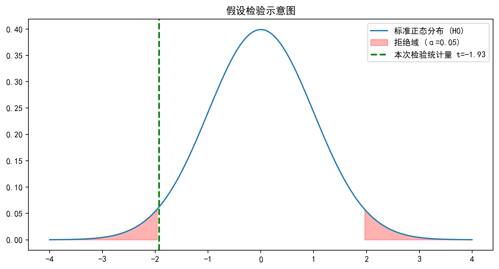
图 5.8 直观地展示了本次假设检验的统计决策过程。图中绘制了标准正态分布 \(N(0,1)\) 的概率密度曲线,两端用红色阴影标出了 \(\alpha = 0.05\) 双侧检验的拒绝域(即 \(z < -1.96\) 和 \(z > 1.96\) 的区域),绿色虚线标记了本次检验统计量的位置。可以看到,绿色虚线落在拒绝域的边缘附近但外侧,与临界值1.96非常接近却未能越过——这与 \(p = 0.054\) 略大于0.05的数值结果完全一致。此图生动地诠释了”统计显著性”的边界决策本质:统计检验并非对效应有无的绝对判定,而是基于预设阈值的概率决策。当检验统计量恰好落在临界值附近时,更应结合效应量和实际商业价值做出综合判断,而非机械地依赖 \(p < 0.05\) 的二元判断。
图 5.8 vividly illustrates the statistical decision-making process of this hypothesis test. The figure plots the probability density curve of the standard normal distribution \(N(0,1)\), with the rejection regions for the two-sided \(\alpha = 0.05\) test shaded in red at both tails (i.e., the areas where \(z < -1.96\) and \(z > 1.96\)), and a green dashed line marks the position of the test statistic. As can be seen, the green dashed line falls near but outside the edge of the rejection region, very close to the critical value of 1.96 yet failing to cross it—entirely consistent with the numerical result of \(p = 0.054\) being slightly greater than 0.05. This figure eloquently illustrates the boundary-decision nature of “statistical significance”: hypothesis testing is not an absolute determination of whether an effect exists, but rather a probabilistic decision based on a preset threshold. When the test statistic happens to fall near the critical value, one should make a comprehensive judgment by combining the effect size and actual business value, rather than mechanically relying on the binary criterion of \(p < 0.05\).
本章从点估计与区间估计出发,系统介绍了推断统计学的核心方法体系。我们首先通过最大似然估计(MLE)建立了参数估计的理论基础,然后深入讲解了置信区间的构造原理与频率学派解释,并通过长三角上市公司的真实财务数据演示了单样本t检验和双样本Welch t检验的完整流程。在启发式思考题中,我们通过蒙特卡洛模拟揭示了p值黑客、样本量与统计显著性的复杂关系,以及t分布对小样本推断的关键保护作用。这些内容为后续章节中更高级的统计建模方法——包括拟合优度检验、方差分析和回归分析——奠定了坚实的推断统计基础。
This chapter began with point estimation and interval estimation, systematically introducing the core methodological framework of inferential statistics. We first established the theoretical foundations of parameter estimation through maximum likelihood estimation (MLE), then provided an in-depth explanation of the construction principles and frequentist interpretation of confidence intervals, and demonstrated the complete workflow of one-sample t-tests and two-sample Welch t-tests using real financial data from Yangtze River Delta listed companies. In the heuristic exercises, we used Monte Carlo simulations to reveal the complex relationships among p-hacking, sample size, and statistical significance, as well as the critical protective role of the t-distribution for small-sample inference. These topics lay a solid inferential statistics foundation for the more advanced statistical modeling methods covered in subsequent chapters—including goodness-of-fit tests, analysis of variance, and regression analysis.