# ========== 导入所需库 ==========
# ========== Import required libraries ==========
import pandas as pd                        # 数据分析库
# Import the pandas library for data analysis
import numpy as np                          # 数值计算库
# Import the numpy library for numerical computation
from scipy.stats import chisquare          # 卡方拟合优度检验函数
# Import the chi-square goodness-of-fit test function
import platform                             # 操作系统检测
# Import the platform module for OS detection
from pathlib import Path                    # 跨平台路径处理
# Import Path for cross-platform path handling

# ========== 第1步:设置本地数据路径 ==========
# ========== Step 1: Set local data path ==========
if platform.system() == 'Windows':                                          # Windows系统路径
    # Windows system path
    data_directory_path = Path('C:/qiufei/data/stock')                     # 设置Windows本地股票数据目录
    # Set the Windows local stock data directory
else:                                                                       # Linux系统路径
    # Linux system path
    data_directory_path = Path('/home/ubuntu/r2_data_mount/qiufei/data/stock')  # 设置Linux本地股票数据目录
    # Set the Linux local stock data directory

# ========== 第2步:读取上市公司基本信息 ==========
# ========== Step 2: Read basic information of listed companies ==========
stock_basic_info_file_path = data_directory_path / 'stock_basic_data.h5'     # 构造文件路径
# Construct the file path
stock_basic_info_dataframe = pd.read_hdf(stock_basic_info_file_path)           # 加载HDF5数据
# Load the HDF5 data

# ========== 第3步:筛选长三角地区企业 ==========
# ========== Step 3: Filter companies in the Yangtze River Delta ==========
yangtze_river_delta_provinces_list = ['上海市', '浙江省', '江苏省']                  # 长三角三省市
# List of three YRD provinces/municipalities
yangtze_river_delta_companies_dataframe = stock_basic_info_dataframe[              # 按省份筛选
    # Filter by province
    stock_basic_info_dataframe['province'].isin(yangtze_river_delta_provinces_list)  # 保留省份在长三角列表中的行
    # Keep rows where the province is in the YRD list
]6 拟合优度检验与列联表分析 (Goodness-of-Fit Tests and Contingency Table Analysis)
本章介绍卡方检验(Chi-Square Test)及其在分类数据分析中的应用。卡方检验是检验分类变量关联性和分布拟合优度的重要工具,广泛应用于市场研究、生物统计、质量控制等领域。
This chapter introduces the Chi-Square Test and its applications in the analysis of categorical data. The chi-square test is an important tool for examining the association between categorical variables and the goodness of fit of distributions, and is widely used in market research, biostatistics, quality control, and other fields.
6.1 拟合优度与独立性检验在金融分析中的典型应用 (Typical Applications of Goodness-of-Fit and Independence Tests in Financial Analysis)
卡方检验在金融和经济研究中用于分析分类变量之间的关联性,以及检验实际数据是否符合理论分布。以下展示其在中国资本市场中的核心应用。
The chi-square test is used in financial and economic research to analyze the association between categorical variables and to test whether observed data conform to a theoretical distribution. The following demonstrates its core applications in China’s capital markets.
6.1.1 应用一:行业分类与财务绩效的独立性检验 (Application 1: Independence Test Between Industry Classification and Financial Performance)
投资研究中一个基本问题是:行业分类是否与公司财务绩效存在显著关联?利用 stock_basic_data.h5 中的行业分类和 financial_statement.h5 中的盈利数据,可以将ROE按分位数划分为”优”、“中”、“差”三类,构建行业×绩效等级的列联表,然后使用卡方独立性检验判断行业归属与盈利水平之间是否存在统计上的显著关联。如果拒绝独立性假设,则意味着行业选择本身就是投资收益的重要决定因素。
A fundamental question in investment research is: Is there a significant association between industry classification and corporate financial performance? Using the industry classifications from stock_basic_data.h5 and profitability data from financial_statement.h5, one can classify ROE into three tiers—“high,” “medium,” and “low”—by quantiles, construct an industry × performance tier contingency table, and then apply a chi-square independence test to determine whether there is a statistically significant association between industry affiliation and profitability level. If the independence hypothesis is rejected, it implies that industry selection itself is an important determinant of investment returns.
6.1.2 应用二:收益率分布的拟合优度检验 (Application 2: Goodness-of-Fit Test for Return Distributions)
检验A股收益率是否服从正态分布是金融风险管理中的基础问题。通过对 stock_price_pre_adjusted.h5 中的日收益率数据进行分组,然后使用卡方拟合优度检验比较实际频率与理论正态分布的预期频率,可以严格量化收益率偏离正态分布的程度。这一检验的结果直接影响VaR模型和期权定价模型的选择(参见 章节 4 中对厚尾分布的讨论)。
Testing whether A-share stock returns follow a normal distribution is a fundamental issue in financial risk management. By grouping daily return data from stock_price_pre_adjusted.h5 and then using the chi-square goodness-of-fit test to compare observed frequencies with the expected frequencies under a theoretical normal distribution, one can rigorously quantify the degree to which returns deviate from normality. The results of this test directly influence the choice of VaR models and option pricing models (see the discussion of heavy-tailed distributions in 章节 4).
6.1.3 应用三:市场微观结构中的交易行为分析 (Application 3: Trading Behavior Analysis in Market Microstructure)
在市场微观结构研究中,卡方检验可用于分析交易行为是否存在显著的时间模式(如”周末效应”、“月初效应”)。通过构建”交易日类型×涨跌方向”的列联表,检验涨跌概率是否在不同时段间保持独立,可以为量化交易策略提供统计依据。
In market microstructure research, the chi-square test can be used to analyze whether trading behavior exhibits significant temporal patterns (such as the “weekend effect” or “turn-of-the-month effect”). By constructing a contingency table of “trading day type × price movement direction” and testing whether the probability of price increases or decreases remains independent across different time periods, one can provide a statistical basis for quantitative trading strategies.
6.2 卡方分布 (The Chi-Square Distribution)
6.2.1 定义与性质 (Definition and Properties)
卡方分布是连续概率分布,是独立标准正态随机变量平方和的分布。
The chi-square distribution is a continuous probability distribution that represents the distribution of the sum of squares of independent standard normal random variables.
定义: 若 \(Z_1, Z_2, ..., Z_k\) 是相互独立的标准正态随机变量,则:
Definition: If \(Z_1, Z_2, ..., Z_k\) are mutually independent standard normal random variables, then:
\[ X = Z_1^2 + Z_2^2 + \cdots + Z_k^2 \]
服从自由度为 \(k\) 的卡方分布,记为 \(X \sim \chi^2(k)\)。
follows a chi-square distribution with \(k\) degrees of freedom, denoted as \(X \sim \chi^2(k)\).
重要性质:
Important Properties:
可加性: 若 \(X_1 \sim \chi^2(k_1)\), \(X_2 \sim \chi^2(k_2)\) 且相互独立,则 \(X_1 + X_2 \sim \chi^2(k_1 + k_2)\)
Additivity: If \(X_1 \sim \chi^2(k_1)\), \(X_2 \sim \chi^2(k_2)\) and they are mutually independent, then \(X_1 + X_2 \sim \chi^2(k_1 + k_2)\)
均值与方差:
- 均值: \(E[X] = k\)
- 方差: \(\text{Var}(X) = 2k\)
Mean and Variance:
- Mean: \(E[X] = k\)
- Variance: \(\text{Var}(X) = 2k\)
与正态分布的关系: 当 \(k\) 很大时(\(k > 30\)), \(\sqrt{2\chi^2(k)}\) 近似服从 \(N(\sqrt{2k-1}, 1)\)
Relationship with the Normal Distribution: When \(k\) is large (\(k > 30\)), \(\sqrt{2\chi^2(k)}\) approximately follows \(N(\sqrt{2k-1}, 1)\)
形状: 卡方分布右偏,自由度越小越偏;随着自由度增加,逐渐接近正态分布
Shape: The chi-square distribution is right-skewed; the smaller the degrees of freedom, the greater the skewness. As the degrees of freedom increase, it gradually approaches the normal distribution.
6.2.2 自由度的含义 (The Meaning of Degrees of Freedom)
自由度(Degrees of Freedom, df)是统计学中一个极其重要但也常常令初学者困惑的概念。简单来说,自由度是指在计算某个统计量时,可以自由取值的独立信息的个数。
Degrees of Freedom (df) is an extremely important concept in statistics that often confuses beginners. Simply put, degrees of freedom refers to the number of independent pieces of information that are free to vary when computing a statistic.
直观理解:约束与自由
Intuitive Understanding: Constraints and Freedom
想象你有5个数,我告诉你它们的平均值是10(即总和为50)。那么:
Imagine you have 5 numbers, and I tell you their mean is 10 (i.e., the sum is 50). Then:
第1个数你可以任意选(比如选8)
第2个数你也可以任意选(比如选12)
第3个数你也可以任意选(比如选9)
第4个数你也可以任意选(比如选11)
但第5个数你没有选择余地——它只能是 \(50 - 8 - 12 - 9 - 11 = 10\)
The 1st number can be freely chosen (say, 8)
The 2nd number can also be freely chosen (say, 12)
The 3rd number can also be freely chosen (say, 9)
The 4th number can also be freely chosen (say, 11)
But the 5th number is fully determined—it can only be \(50 - 8 - 12 - 9 - 11 = 10\)
换句话说,在”总和=50”这一约束条件下,5个数中只有4个能自由变化,最后一个被自动确定了。因此自由度为 \(df = 5 - 1 = 4\)。
In other words, under the constraint “sum = 50,” only 4 of the 5 numbers can vary freely; the last one is automatically determined. Therefore, the degrees of freedom is \(df = 5 - 1 = 4\).
一般原则:如果有 \(n\) 个独立的观测值,每施加一个约束(如估计一个参数),就会”消耗”一个自由度。最终的自由度 = 观测值个数 – 施加的约束个数。
General Principle: If there are \(n\) independent observations, each constraint imposed (such as estimating a parameter) “consumes” one degree of freedom. The final degrees of freedom = number of observations – number of constraints imposed.
为什么自由度在统计推断中至关重要?
Why Are Degrees of Freedom Critical in Statistical Inference?
自由度直接决定了检验统计量的抽样分布。以卡方检验为例,同样的 \(\chi^2 = 10\),在 \(df = 2\) 时对应极小的 \(p\) 值(强烈拒绝原假设),而在 \(df = 10\) 时对应较大的 \(p\) 值(不拒绝原假设)。如果自由度计算错误,整个统计推断的结论都会出错。
Degrees of freedom directly determine the sampling distribution of the test statistic. Taking the chi-square test as an example, the same \(\chi^2 = 10\) corresponds to a very small \(p\)-value at \(df = 2\) (strongly rejecting the null hypothesis), but a much larger \(p\)-value at \(df = 10\) (failing to reject the null hypothesis). If the degrees of freedom are calculated incorrectly, the conclusions of the entire statistical inference will be wrong.
在卡方检验中的自由度
Degrees of Freedom in Chi-Square Tests
在卡方检验中,自由度的计算规则如下:
The rules for calculating degrees of freedom in chi-square tests are as follows:
拟合优度检验: \(df = k - 1 - m\),其中 \(k\) 是类别数,\(m\) 是从数据中估计的参数个数
独立性检验: \(df = (r-1)(c-1)\),其中 \(r\) 和 \(c\) 分别是行数和列数
Goodness-of-fit test: \(df = k - 1 - m\), where \(k\) is the number of categories and \(m\) is the number of parameters estimated from the data
Independence test: \(df = (r-1)(c-1)\), where \(r\) and \(c\) are the number of rows and columns, respectively
为什么拟合优度检验中 \(df = k - 1 - m\)?
Why Is \(df = k - 1 - m\) in the Goodness-of-Fit Test?
首先,\(k\) 个类别的频数之和等于总样本量 \(n\),这是一个固有约束,因此从 \(k\) 个频数中必须减去1,得到 \(k-1\) 个自由变化的频数。
其次,如果我们还从数据中估计了分布的参数(比如正态分布的均值 \(\mu\) 和方差 \(\sigma^2\)),每估计一个参数就相当于施加了额外的约束,每个参数再减去1个自由度。所以最终 \(df = k - 1 - m\)。
First, the sum of frequencies across \(k\) categories equals the total sample size \(n\), which is an inherent constraint. Therefore, 1 must be subtracted from \(k\) frequencies, yielding \(k-1\) freely varying frequencies.
Second, if we additionally estimate distribution parameters from the data (such as the mean \(\mu\) and variance \(\sigma^2\) of a normal distribution), each estimated parameter imposes an additional constraint, reducing the degrees of freedom by 1 for each parameter. Thus, the final result is \(df = k - 1 - m\).
为什么独立性检验中 \(df = (r-1)(c-1)\)?
Why Is \(df = (r-1)(c-1)\) in the Independence Test?
列联表有 \(r \times c\) 个单元格,但行合计(\(r\) 个约束,因给定列总数后只有 \(r-1\) 个独立)和列合计(\(c-1\) 个独立约束)加上总样本量的约束,使得最终可自由变化的单元格数为 \((r-1)(c-1)\)。
A contingency table has \(r \times c\) cells, but the row totals (\(r\) constraints, of which only \(r-1\) are independent given the column totals) and column totals (\(c-1\) independent constraints), together with the constraint on the total sample size, result in \((r-1)(c-1)\) freely varying cells.
6.3 卡方拟合优度检验 (Chi-Square Goodness-of-Fit Test)
6.3.1 检验原理 (Test Principle)
拟合优度检验用于检验观测频数是否符合理论分布。
The goodness-of-fit test is used to test whether observed frequencies conform to a theoretical distribution.
假设设置:
Hypothesis Setup:
原假设 \(H_0\): 观测数据服从理论分布
备择假设 \(H_1\): 观测数据不服从理论分布
Null hypothesis \(H_0\): The observed data follow the theoretical distribution
Alternative hypothesis \(H_1\): The observed data do not follow the theoretical distribution
卡方统计量:
Chi-Square Statistic:
如 式 6.1 所示,卡方统计量的计算公式为:
As shown in 式 6.1, the formula for the chi-square statistic is:
\[ \chi^2 = \sum_{i=1}^{k} \frac{(O_i - E_i)^2}{E_i} \tag{6.1}\]
其中:
Where:
\(O_i\): 第 \(i\) 类别的观测频数
\(E_i\): 第 \(i\) 类别的理论频数
\(O_i\): Observed frequency in the \(i\)-th category
\(E_i\): Expected (theoretical) frequency in the \(i\)-th category
6.3.2 卡方统计量的数学本质 (The Mathematical Essence of the Chi-Square Statistic)
为什么 \(\sum \frac{(O-E)^2}{E}\) 会服从卡方分布? 这源于正态近似。
Why does \(\sum \frac{(O-E)^2}{E}\) follow a chi-square distribution? This stems from the normal approximation.
考虑第 \(i\) 个类别的观测频数 \(O_i\)。根据二项分布,它的期望是 \(E_i = np_i\),方差是 \(Var(O_i) = np_i(1-p_i) \approx np_i = E_i\)(当 \(p_i\) 很小时,泊松近似)。
Consider the observed frequency \(O_i\) for the \(i\)-th category. According to the binomial distribution, its expectation is \(E_i = np_i\), and its variance is \(Var(O_i) = np_i(1-p_i) \approx np_i = E_i\) (under the Poisson approximation when \(p_i\) is small).
我们将 \(O_i\) 标准化:
We standardize \(O_i\):
\[ Z_i = \frac{O_i - E_i}{\sqrt{Var(O_i)}} \approx \frac{O_i - E_i}{\sqrt{E_i}} \]
将它们平方并求和:
Squaring and summing them:
\[ \chi^2 = \sum Z_i^2 = \sum \frac{(O_i - E_i)^2}{E_i} \]
这也是为什么卡方检验要求样本量大(保证正态近似有效)且理论频数 \(E_i\) 不能太小(作为分母,太小会导致统计量不稳定)。
This is also why the chi-square test requires a large sample size (to ensure the validity of the normal approximation) and that the expected frequencies \(E_i\) not be too small (as the denominator, very small values would make the statistic unstable).
直观理解:
Intuitive Understanding:
\(\chi^2\) 实际上是标准化残差的平方和。
它衡量了观测数据与理论模型之间的”欧几里得距离”。
\(\chi^2\) is essentially the sum of squared standardized residuals.
It measures the “Euclidean distance” between the observed data and the theoretical model.
6.3.3 适用条件 (Conditions for Applicability)
卡方检验的有效性依赖于以下条件:
The validity of the chi-square test depends on the following conditions:
样本量足够大: 每个类别的理论频数 \(E_i \geq 5\)
- 如果某些类别频数过小,可合并相邻类别
- 或使用精确检验(Fisher’s Exact Test)
Sufficiently large sample size: The expected frequency for each category \(E_i \geq 5\)
- If some categories have frequencies that are too small, adjacent categories can be merged
- Or an exact test (Fisher’s Exact Test) can be used
数据独立: 每个观测相互独立
- 不能有重复测量或配对数据
Independence of data: Each observation is mutually independent
- No repeated measures or paired data are allowed
互斥且穷尽: 每个观测只能落入一个类别,且所有类别覆盖全部可能
Mutually exclusive and exhaustive: Each observation can fall into only one category, and all categories cover every possibility
6.3.4 检验步骤 (Testing Procedure)
- 建立假设: 明确原假设和备择假设
- 计算理论频数: 根据 \(H_0\) 计算每个类别的期望频数
- 计算卡方统计量: 使用公式计算 \(\chi^2\)
- 确定自由度: \(df = k - 1 - m\)
- 查找临界值或计算p值: 与 \(\chi^2\) 分布比较
- 做出决策:
- 若 \(p < \alpha\),拒绝 \(H_0\)
- 若 \(p \geq \alpha\),不能拒绝 \(H_0\)
- Formulate hypotheses: Clearly state the null and alternative hypotheses
- Compute expected frequencies: Calculate expected frequencies for each category under \(H_0\)
- Compute the chi-square statistic: Use the formula to calculate \(\chi^2\)
- Determine degrees of freedom: \(df = k - 1 - m\)
- Find the critical value or compute the p-value: Compare with the \(\chi^2\) distribution
- Make a decision:
- If \(p < \alpha\), reject \(H_0\)
- If \(p \geq \alpha\), fail to reject \(H_0\)
6.3.5 优缺点 (Advantages and Disadvantages)
优点:
Advantages:
非参数方法:不假设数据服从特定连续分布,适用范围广
计算简单:公式直观,只需观测频数和理论频数
检验有力:对分布偏离的检测功效较高
Nonparametric method: Does not assume the data follow a specific continuous distribution; broadly applicable
Computationally simple: The formula is intuitive, requiring only observed and expected frequencies
Powerful test: Has relatively high power for detecting distributional deviations
缺点:
Disadvantages:
对小样本敏感:要求 \(E_i \geq 5\),否则近似不可靠
信息损失:将连续变量分箱会丢失精确信息
方向性不明:只能告诉你”不符合”,不能告诉你”如何不符合”(需要看标准化残差)
对分箱方案敏感:不同的分箱方案可能导致不同结论
Sensitive to small samples: Requires \(E_i \geq 5\); otherwise the approximation is unreliable
Information loss: Binning continuous variables results in loss of precise information
Lack of directionality: Can only tell you “does not fit,” not “how it does not fit” (standardized residuals must be examined)
Sensitive to binning scheme: Different binning schemes may lead to different conclusions
6.3.6 “脏活累活” (Dirty Work):分箱的艺术 (The Art of Binning)
卡方检验最头疼的问题往往不是算 \(p\) 值,而是如何分箱 (Binning)。
The most troublesome issue with the chi-square test is often not computing the \(p\)-value, but rather how to bin the data (Binning).
对于连续变量(如年龄、收入),我们需要先将其离散化。
For continuous variables (such as age or income), we need to discretize them first.
分箱太细:会导致很多格子 \(E_i < 5\),统计检验失效。
分箱太粗:会掩盖数据内部的分布特征(例如把 10-20岁 和 20-60岁 合并,就看不出青年人的特征)。
Too fine: Leads to many cells with \(E_i < 5\), causing the statistical test to break down.
Too coarse: Masks the internal distribution characteristics of the data (e.g., merging 10–20 years old and 20–60 years old makes it impossible to see the characteristics of young people).
黄金法则:
Golden Rules:
理论优先:根据业务逻辑分箱(如:未成年/青年/中年/老年)。
等频分箱:确保每个箱子的样本量大致相等,最大化统计功效。
合并稀疏项:一旦发现某个格子 \(E_i < 5\),哪怕违背业务逻辑,也要将其与相邻格子合并。因为统计有效性是底线。
Theory first: Bin according to business logic (e.g., minor / young adult / middle-aged / elderly).
Equal-frequency binning: Ensure each bin contains roughly the same number of observations to maximize statistical power.
Merge sparse cells: Once a cell with \(E_i < 5\) is found, it must be merged with an adjacent cell, even if it violates business logic, because statistical validity is the baseline requirement.
6.3.7 案例:长三角地区行业分布检验 (Case Study: Industry Distribution Test in the Yangtze River Delta)
什么是行业分布的均匀性检验?
What Is a Uniformity Test for Industry Distribution?
区域经济研究和产业规划中,一个关键问题是:某个地区的产业结构是否均衡,还是存在明显的行业集中化现象?例如,长三角地区是中国经济最活跃的区域之一,其上市公司的行业分布是否均匀,直接反映了该区域的产业多元化程度和经济结构特征。
In regional economic research and industrial planning, a key question is: Is the industrial structure of a given region balanced, or does it exhibit significant industry concentration? For example, the Yangtze River Delta (YRD) is one of the most economically active regions in China, and whether its listed companies are evenly distributed across industries directly reflects the region’s degree of industrial diversification and economic structural characteristics.
卡方拟合优度检验是解决此类问题的经典统计工具:它将观察到的各行业公司数量与「均匀分布」假设下的期望数量进行比较,如果实际分布与均匀分布差异显著,则说明存在行业集中化。下面使用本地数据集检验长三角地区不同行业的公司分布是否均匀,结果如 表 6.1 所示。
The chi-square goodness-of-fit test is a classic statistical tool for addressing such questions: it compares the observed number of companies in each industry with the expected numbers under a “uniform distribution” hypothesis. If the actual distribution differs significantly from a uniform distribution, it indicates the presence of industry concentration. Below, we use a local dataset to test whether the distribution of companies across industries in the YRD is uniform, with results shown in 表 6.1.
长三角地区上市公司筛选完毕。下面统计行业分布并输出前5大行业的频数。
The filtering of listed companies in the YRD is complete. Next, we compute the industry distribution and output the frequencies of the top 5 industries.
# ========== 第4步:统计行业分布并取前5大行业 ==========
# ========== Step 4: Compute industry distribution and select the top 5 industries ==========
industry_frequency_counts_series = yangtze_river_delta_companies_dataframe[        # 计算各行业频数
    # Compute the frequency for each industry
    'industry_name'                                                                # 选取行业名称列
    # Select the industry name column
].value_counts()                                                                  # 统计各行业出现频次并降序排列
# Count the frequency of each industry and sort in descending order
top_five_industries_series = industry_frequency_counts_series.head(5)              # 选取前5大行业
# Select the top 5 industries

print('=' * 60)                                                                 # 打印分隔线
# Print a separator line
print('长三角地区上市公司行业分布')                                                   # 输出标题
# Print the title
print('=' * 60)                                                                 # 打印分隔线
# Print a separator line
print('\n观测频数:')                                                               # 提示下方为频数数据
# Indicate that observed frequencies follow
print(top_five_industries_series)                                                 # 输出前5行业的频数统计
# Print the frequency statistics for the top 5 industries
============================================================
长三角地区上市公司行业分布
============================================================
观测频数:
industry_name
计算机、通信和其他电子设备制造业 180
电气机械和器材制造业 150
专用设备制造业 146
化学原料和化学制品制造业 131
通用设备制造业 118
Name: count, dtype: int64长三角地区前5大行业的观测频数统计结果显示:计算机、通信和其他电子设备制造业以180家公司位居榜首,其后依次为电气机械和器材制造业(150家)、专用设备制造业(146家)、化学原料和化学制品制造业(131家)和通用设备制造业(118家),5个行业合计725家。从直觉上看,这5个行业的公司数量并非完全均等,计算机通信行业明显偏多,而通用设备行业偏少。下面构建均匀分布假设下的期望频数并执行卡方拟合优度检验,用统计方法严格判断这种差异是否达到了显著水平。
The observed frequency statistics for the top 5 industries in the YRD show that Computer, Communication and Other Electronic Equipment Manufacturing ranks first with 180 companies, followed by Electrical Machinery and Equipment Manufacturing (150), Special-Purpose Equipment Manufacturing (146), Chemical Raw Materials and Chemical Products Manufacturing (131), and General-Purpose Equipment Manufacturing (118), totaling 725 companies across the 5 industries. Intuitively, the number of companies across these 5 industries is not perfectly equal—the computer and communications industry is notably overrepresented, while general-purpose equipment is underrepresented. Next, we construct the expected frequencies under the uniform distribution hypothesis and perform a chi-square goodness-of-fit test to rigorously determine whether this difference reaches statistical significance.
# ========== 第5步:构建均匀分布假设下的期望频数 ==========
# ========== Step 5: Construct expected frequencies under the uniform distribution hypothesis ==========
total_companies_in_top_sectors_count = top_five_industries_series.sum()                # 前5行业公司总数
# Total number of companies in the top 5 industries
uniform_expected_frequency_value = (                                                   # 均匀分布下每行业期望数
    # Expected number per industry under uniform distribution
    total_companies_in_top_sectors_count / len(top_five_industries_series)              # 总数除以行业数得到均值
    # Divide total by the number of industries to get the mean
)
expected_frequencies_list = [uniform_expected_frequency_value] * len(                  # 构造期望频数列表
    # Construct the list of expected frequencies
    top_five_industries_series                                                         # 列表长度与行业数一致
    # List length matches the number of industries
)

# ========== 第6步:执行卡方拟合优度检验 ==========
# ========== Step 6: Perform the chi-square goodness-of-fit test ==========
chi_square_statistic_value, calculated_p_value = chisquare(                           # scipy卡方检验
    # Perform the scipy chi-square test
    top_five_industries_series.values, f_exp=expected_frequencies_list                  # 传入观测频数和期望频数
    # Pass in observed frequencies and expected frequencies
)
degrees_of_freedom_value = len(top_five_industries_series) - 1                        # 自由度 = 类别数 - 1
# Degrees of freedom = number of categories - 1

print(f'\n原假设 H0: 各行业公司数量相等')                                             # 输出原假设
# Print the null hypothesis
print(f'备择假设 H1: 各行业公司数量不相等')                                           # 输出备择假设
# Print the alternative hypothesis
print(f'\n卡方统计量: {chi_square_statistic_value:.4f}')                              # 输出χ²统计量
# Print the chi-square statistic
print(f'自由度: {degrees_of_freedom_value}')                                          # 输出自由度
# Print the degrees of freedom
print(f'p值: {calculated_p_value:.8f}')                                               # 输出p值
# Print the p-value
原假设 H0: 各行业公司数量相等
备择假设 H1: 各行业公司数量不相等

卡方统计量: 15.0069
自由度: 4
p值: 0.00468693卡方检验结果为:\(\chi^2 = 15.0069\),自由度 \(df = 4\),\(p = 0.00469\)。在均匀分布的原假设下,每个行业的期望频数为 \(725/5 = 145\) 家。\(p\) 值远小于显著性水平0.05,说明我们有充分的统计学证据拒绝”各行业公司数量相等”的原假设——长三角地区前5大行业的公司数量分布确实不均匀。下面进行显著性判断并计算标准化残差,以识别偏离均匀分布最大的行业。
The chi-square test results are: \(\chi^2 = 15.0069\), degrees of freedom \(df = 4\), and \(p = 0.00469\). Under the null hypothesis of a uniform distribution, the expected frequency for each industry is \(725/5 = 145\) companies. The \(p\)-value is far below the significance level of 0.05, indicating that we have sufficient statistical evidence to reject the null hypothesis that “all industries have equal numbers of companies”—the distribution of companies across the top 5 industries in the YRD is indeed non-uniform. Next, we assess statistical significance and compute standardized residuals to identify the industries that deviate most from the uniform distribution.
# ========== 第7步:统计显著性判断 ==========
# ========== Step 7: Statistical significance assessment ==========
significance_level_alpha = 0.05                                                        # 显著性水平 α=0.05
# Significance level α = 0.05
print(f'\n结论 (α={significance_level_alpha}):')                                       # 输出显著性判断标题
# Print the significance assessment heading
if calculated_p_value < significance_level_alpha:                                      # p < α 则拒绝H0
    # If p < α, reject H0
    print(f'  拒绝H0 (p={calculated_p_value:.8f} < {significance_level_alpha})')      # 输出拒绝原假设结论
    # Print the conclusion of rejecting the null hypothesis
    print(f'  各行业公司数量存在显著差异,分布不均匀')                                   # 说明行业分布不均匀
    # State that significant differences exist among industries; the distribution is non-uniform
else:                                                                                  # p ≥ α 则不拒绝H0
    # If p ≥ α, fail to reject H0
    print(f'  不能拒绝H0 (p={calculated_p_value:.8f} >= {significance_level_alpha})')  # 输出不拒绝结论
    # Print the conclusion of failing to reject the null hypothesis
    print(f'  没有证据表明各行业公司数量不均衡')                                       # 说明无显著差异
    # State that there is no evidence of imbalance among industries

# ========== 第8步:计算标准化残差(识别偏离最大的类别) ==========
# ========== Step 8: Compute standardized residuals (identify the most deviant categories) ==========
observed_frequencies_array = top_five_industries_series.values                          # 观测频数数组
# Array of observed frequencies
standardized_residuals_array = (                                                        # 标准化残差=(O-E)/√E
    # Standardized residuals = (O - E) / √E
    (observed_frequencies_array - uniform_expected_frequency_value)                      # 计算观测与期望的偏差
    # Compute the deviation between observed and expected
    / np.sqrt(uniform_expected_frequency_value)                                         # 除以期望频数的平方根进行标准化
    # Divide by the square root of the expected frequency for standardization
)

print(f'\n标准化残差:')                                                                # 输出残差表头
# Print the residuals heading
for industry_name, residual_value in zip(                                              # 逐行业输出残差
    # Output residuals for each industry
    top_five_industries_series.index, standardized_residuals_array                      # 配对行业名与残差值
    # Pair industry names with residual values
):
    print(f'  {industry_name}: {residual_value:.3f}')                                  # 逐行输出行业名及其残差
    # Print each industry name and its residual
结论 (α=0.05):
  拒绝H0 (p=0.00468693 < 0.05)
  各行业公司数量存在显著差异,分布不均匀

标准化残差:
  计算机、通信和其他电子设备制造业: 2.907
  电气机械和器材制造业: 0.415
  专用设备制造业: 0.083
  化学原料和化学制品制造业: -1.163
  通用设备制造业: -2.242
表 6.1 的结果证实了我们的判断:在 \(\alpha = 0.05\) 水平下拒绝原假设(\(p = 0.00469\)),各行业公司数量存在显著差异。标准化残差揭示了偏离的具体方向——计算机、通信行业的残差为 +2.907(绝对值超过2,属于显著偏多),这反映了长三角地区作为中国电子信息产业集聚高地的实际情况;通用设备制造业的残差为 -2.242(显著偏少),说明该行业在长三角的集聚程度相对较低。电气机械(+0.415)、专用设备(+0.083)和化学原料(-1.163)的残差绝对值均未超过2,偏离不显著。这一分析为理解区域产业结构特征提供了定量依据。
The results in 表 6.1 confirm our assessment: at the \(\alpha = 0.05\) level, the null hypothesis is rejected (\(p = 0.00469\)), indicating significant differences in the number of companies across industries. The standardized residuals reveal the specific direction of deviation—the Computer and Communications industry has a residual of +2.907 (absolute value exceeding 2, indicating significantly more companies than expected), reflecting the YRD’s status as a major hub for China’s electronic information industry. The General-Purpose Equipment Manufacturing industry has a residual of -2.242 (significantly fewer than expected), indicating a relatively lower degree of concentration for this industry in the YRD. The residuals for Electrical Machinery (+0.415), Special-Purpose Equipment (+0.083), and Chemical Raw Materials (-1.163) all have absolute values below 2, indicating non-significant deviations. This analysis provides a quantitative basis for understanding regional industrial structure characteristics. ## 从理论到实践:苦活累活 (The “Dirty Work”) {#sec-dirty-work-ch6}
6.4 From Theory to Practice: The “Dirty Work”
卡方检验看似简单,但在实际操作中,它比你想象的要”脏”得多。
The chi-square test may seem simple, but in practice it is much “dirtier” than you might expect.
6.4.1 1. 分箱黑客 (Binning Hacking)
当处理连续变量(如年龄、收入)时,我们需要先将其离散化(分箱)。 - 问题:P值高度依赖于你如何分箱。 - 黑客手段:如果你想要显著结果,就把箱子分得细一点;如果你想要不显著,就把箱子合并一下。通过调整分箱边界(如 10-20岁 改为 10-18岁),你可以轻松”操纵”P值。 - 防御:这就叫 Multiverse Analysis(多重宇宙分析)。诚实的研究者应该报告多种分箱方案下的结果,看结论是否稳健。
When dealing with continuous variables (such as age or income), we first need to discretize (bin) them. - Problem: The P-value is highly dependent on how you bin the data. - Hacking technique: If you want a significant result, make the bins finer; if you want non-significance, merge the bins. By adjusting bin boundaries (e.g., changing 10–20 years old to 10–18 years old), you can easily “manipulate” the P-value. - Defense: This is called Multiverse Analysis. Honest researchers should report results under multiple binning schemes and check whether the conclusions are robust.
6.4.2 2. 样本量的诅咒 (The Curse of Large N)
卡方检验对样本量极其敏感。 - 当 \(N\) 很大(如互联网数据中的百万级用户)时,即使是微不足道的偏差(如 0.1% 的差异),也会产生极小的 P值(P < 0.0001)。 - 后果:你会发现”一切都显著”,但这毫无意义。 - 对策:在大样本下,忘掉 P值,只看 Cramer’s V(效应量)。如果 \(V < 0.1\),哪怕 \(P\) 再小,这个关联也是微不足道的。
The chi-square test is extremely sensitive to sample size. - When \(N\) is large (e.g., millions of users in internet data), even trivial deviations (such as a 0.1% difference) can produce extremely small P-values (P < 0.0001). - Consequence: You will find that “everything is significant,” but it is meaningless. - Countermeasure: With large samples, forget the P-value and look only at Cramer’s V (effect size). If \(V < 0.1\), no matter how small \(P\) is, the association is negligible.
6.5 列联表与独立性检验 (Contingency Tables and Independence Tests)
6.5.1 列联表结构 (Structure of Contingency Tables)
列联表(Contingency Table)是两个或多个分类变量的交叉频数表。对于两个变量,其结构如下:
A contingency table is a cross-tabulation of frequencies for two or more categorical variables. For two variables, its structure is as follows:
| 列1 | 列2 | … | 列c | 行合计 | |
|---|---|---|---|---|---|
| 行1 | O₁₁ | O₁₂ | … | O₁c | R₁ |
| 行2 | O₂₁ | O₂₂ | … | O₂c | R₂ |
| … | … | … | … | … | … |
| 行r | Or₁ | Or₂ | … | Orc | Rr |
| 列合计 | C₁ | C₂ | … | Cc | n |
其中 \(O_{ij}\) 是第 \(i\) 行第 \(j\) 列的观测频数,\(n\) 是总样本量。
where \(O_{ij}\) is the observed frequency in the \(i\)-th row and \(j\)-th column, and \(n\) is the total sample size.
6.5.2 独立性检验 (Independence Test)
检验两个分类变量是否相互独立。
This test examines whether two categorical variables are independent of each other.
假设设置: - 原假设 \(H_0\): 两个变量相互独立(无关联) - 备择假设 \(H_1\): 两个变量不独立(存在关联)
Hypotheses: - Null hypothesis \(H_0\): The two variables are independent (no association) - Alternative hypothesis \(H_1\): The two variables are not independent (association exists)
理论频数计算:
Calculating Expected Frequencies:
在独立性假设下,第 \((i, j)\) 格的理论频数如 式 6.2 所示:
Under the independence assumption, the expected frequency for cell \((i, j)\) is given by 式 6.2:
\[ E_{ij} = \frac{R_i \times C_j}{n} \tag{6.2}\]
其中 \(R_i\) 和 \(C_j\) 分别是第 \(i\) 行和第 \(j\) 列的边际和。
where \(R_i\) and \(C_j\) are the marginal totals for the \(i\)-th row and \(j\)-th column, respectively.
卡方统计量:
Chi-Square Statistic:
独立性检验的卡方统计量如 式 6.3 所示:
The chi-square statistic for the independence test is shown in 式 6.3:
\[ \chi^2 = \sum_{i=1}^{r} \sum_{j=1}^{c} \frac{(O_{ij} - E_{ij})^2}{E_{ij}} \tag{6.3}\]
自由度: \(df = (r-1)(c-1)\)
Degrees of freedom: \(df = (r-1)(c-1)\)
效应量:
Effect Size:
除了统计显著性,我们还应关注关联强度。常用指标包括:
Beyond statistical significance, we should also examine the strength of association. Common measures include:
Phi系数 (\(\phi\)) (仅适用于 \(2 \times 2\) 表): \[ \phi = \sqrt{\frac{\chi^2}{n}} \]
Phi coefficient (\(\phi\)) (only applicable to \(2 \times 2\) tables): \[ \phi = \sqrt{\frac{\chi^2}{n}} \]
Cramer’s V (适用于任意大小的表): \[ V = \sqrt{\frac{\chi^2}{n \times \min(r-1, c-1)}} \]
Cramer’s V (applicable to tables of any size): \[ V = \sqrt{\frac{\chi^2}{n \times \min(r-1, c-1)}} \]
列联系数 (Contingency Coefficient \(C\)): \[ C = \sqrt{\frac{\chi^2}{\chi^2 + n}} \]
Contingency Coefficient (\(C\)): \[ C = \sqrt{\frac{\chi^2}{\chi^2 + n}} \]
解释: - \(0 \leq \phi, V, C \leq 1\) (对于 \(2 \times 2\) 表) - 值越大,关联越强 - 但这些指标的上限受表的大小影响,不同表之间难以直接比较
Interpretation: - \(0 \leq \phi, V, C \leq 1\) (for \(2 \times 2\) tables) - Larger values indicate stronger association - However, the upper bounds of these measures are affected by table dimensions, making direct comparison across different tables difficult
6.5.3 案例:长三角行业与地区的关联 (Case Study: Industry–Region Association in the Yangtze River Delta)
什么是行业与地区的独立性检验?
What Is an Industry–Region Independence Test?
在区域经济研究中,一个重要的研究问题是:一个地区的优势产业是否与其地理位置相关?例如,浙江是否更偏重信息技术行业,而江苏是否更偏重制造业?这种产业布局的区域差异对于产业政策制定、招商引资战略和投资组合的区域配置都具有重要参考价值。
In regional economic research, an important question is whether a region’s dominant industries are related to its geographic location. For example, does Zhejiang lean more heavily toward the information technology sector, while Jiangsu favors manufacturing? Such regional differences in industrial structure have significant implications for industrial policy-making, investment attraction strategies, and geographic allocation of investment portfolios.
卡方独立性检验能够回答这个问题:它检验两个分类变量(行业和省份)之间是否存在统计上的显著关联。如果检验结果拒绝独立性假设,则说明行业分布确实因地区而异,存在显著的区域产业集群效应。下面使用本地上市公司数据检验长三角地区行业分布与省份是否独立,结果如 表 6.2 所示。
The chi-square independence test can answer this question: it tests whether a statistically significant association exists between two categorical variables (industry and province). If the test rejects the independence hypothesis, it indicates that industry distributions do vary across regions, suggesting significant regional industrial clustering effects. Below we use local listed-company data to test whether the industry distribution in the Yangtze River Delta is independent of province, with results shown in 表 6.2.
# ========== 导入所需库 ==========
# ========== Import required libraries ==========
import pandas as pd                          # 数据分析库
# Import the pandas library for data analysis
import numpy as np                            # 数值计算库
# Import the numpy library for numerical computation
from scipy.stats import chi2_contingency     # 卡方独立性检验函数
# Import the chi-square independence test function
import platform                               # 操作系统检测
# Import the platform module for OS detection
from pathlib import Path                      # 跨平台路径处理
# Import Path for cross-platform path handling

# ========== 第1步:设置本地数据路径 ==========
# ========== Step 1: Set local data path ==========
# 使用本地上市公司数据:检验行业与地区的独立性
# Use local listed-company data: test independence between industry and region
if platform.system() == 'Windows':                                                # Windows系统路径
    # Windows system path
    stock_data_directory_path = Path('C:/qiufei/data/stock')                       # 设置Windows本地股票数据目录
    # Set the Windows local stock data directory
else:                                                                             # Linux系统路径
    # Linux system path
    stock_data_directory_path = Path('/home/ubuntu/r2_data_mount/qiufei/data/stock')  # 设置Linux本地股票数据目录
    # Set the Linux local stock data directory

# ========== 第2步:读取上市公司基本信息 ==========
# ========== Step 2: Load listed-company basic information ==========
stock_basic_info_dataframe = pd.read_hdf(                                     # 加载HDF5格式数据
    # Load data in HDF5 format
    stock_data_directory_path / 'stock_basic_data.h5'                          # 指定上市公司基本信息文件路径
    # Specify the file path for listed-company basic information
)
上市公司基本信息数据加载完毕。下面筛选长三角企业并构建行业×地区列联表。
Listed-company basic information has been loaded. Next, we filter for Yangtze River Delta companies and construct the industry × region contingency table.
# ========== 第3步:筛选长三角三省企业 ==========
# ========== Step 3: Filter companies in the three YRD provinces ==========
yangtze_river_delta_provinces = ['上海市', '浙江省', '江苏省']                       # 长三角三省市
# The three provinces/municipalities of the Yangtze River Delta
yrd_companies_dataframe = stock_basic_info_dataframe[                              # 按省份筛选
    # Filter by province
    stock_basic_info_dataframe['province'].isin(yangtze_river_delta_provinces)      # 保留省份属于长三角的公司
    # Keep companies whose province belongs to the YRD
].copy()                                                                           # 深拷贝避免链式赋值警告
# Deep copy to avoid chained-assignment warnings

# ========== 第4步:选取前4大行业并构建列联表 ==========
# ========== Step 4: Select the top 4 industries and build a contingency table ==========
top_four_industries_list = (                                                       # 获取频数最高的4个行业
    # Get the 4 industries with the highest frequency
    yrd_companies_dataframe['industry_name'].value_counts().head(4).index.tolist()  # 统计行业频次并取前4名
    # Count industry frequencies and take the top 4
)
yrd_top_industry_dataframe = yrd_companies_dataframe[                              # 筛选这4个行业的公司
    # Filter companies in these 4 industries
    yrd_companies_dataframe['industry_name'].isin(top_four_industries_list)         # 保留行业名在前4列表中的公司
    # Keep companies whose industry name is in the top 4 list
]

industry_area_contingency_table = pd.crosstab(                                     # 创建 行业×地区 交叉频数表
    # Create the industry × region cross-tabulation
    yrd_top_industry_dataframe['industry_name'],                                    # 行变量:行业名称
    # Row variable: industry name
    yrd_top_industry_dataframe['province'],                                         # 列变量:省份
    # Column variable: province
    margins=False                                                                  # 不添加边际合计行/列
    # Do not add marginal totals
)

print('=' * 60)                                                                    # 打印分隔线
# Print a separator line
print('行业 vs. 地区 列联表 (长三角上市公司)')                                     # 输出标题
# Print the table title
print('=' * 60)                                                                    # 打印分隔线
# Print a separator line
print(industry_area_contingency_table)                                              # 输出行业与地区的交叉频数表
# Print the industry–region cross-tabulation
============================================================
行业 vs. 地区 列联表 (长三角上市公司)
============================================================
province 上海市 江苏省 浙江省
industry_name
专用设备制造业 32 62 52
化学原料和化学制品制造业 24 60 47
电气机械和器材制造业 23 66 61
计算机、通信和其他电子设备制造业 45 88 47行业与地区的列联表已构建完毕。从列联表中可以初步观察到:计算机、通信行业在上海(45家)和江苏(88家)的集中度较高,而在浙江仅47家;电气机械行业在江苏(66家)和浙江(61家)较为均衡,上海仅23家。这些差异是否具有统计显著性?下面执行卡方独立性检验,计算Cramer’s V效应量和标准化残差,以判断行业分布在长三角三省之间是否存在显著差异。
The contingency table has been constructed. From the table, we can make some preliminary observations: the computer and telecommunications industry shows higher concentration in Shanghai (45 firms) and Jiangsu (88 firms), while only 47 firms are in Zhejiang; the electrical machinery industry is relatively balanced between Jiangsu (66 firms) and Zhejiang (61 firms), with only 23 firms in Shanghai. Are these differences statistically significant? Below we perform the chi-square independence test, calculate Cramer’s V effect size and standardized residuals, to determine whether the industry distribution differs significantly across the three YRD provinces.
# ========== 第5步:执行卡方独立性检验 ==========
# ========== Step 5: Perform the chi-square independence test ==========
chi2_statistic_value, calculated_p_value, degrees_of_freedom_value, expected_frequencies_array = (  # 执行卡方独立性检验
    # Perform the chi-square independence test
    chi2_contingency(industry_area_contingency_table)                              # 返回χ²、p值、df、期望频数
    # Returns χ², p-value, df, and expected frequencies
)

print(f'\n卡方统计量: {chi2_statistic_value:.4f}')                                 # 输出χ²统计量
# Print the χ² statistic
print(f'自由度: {degrees_of_freedom_value}')                                         # 输出自由度
# Print the degrees of freedom
print(f'p值: {calculated_p_value:.6f}')                                              # 输出p值
# Print the p-value

# ========== 第6步:计算Cramer's V效应量 ==========
# ========== Step 6: Calculate the Cramer's V effect size ==========
total_samples_count = industry_area_contingency_table.sum().sum()                  # 总样本量
# Total sample size
minimum_dimension_size = min(                                                      # min(行数, 列数) - 1
    # min(number of rows, number of columns) - 1
    industry_area_contingency_table.shape[0],                                       # 列联表行数
    # Number of rows in the contingency table
    industry_area_contingency_table.shape[1]                                        # 列联表列数
    # Number of columns in the contingency table
) - 1                                                                              # 取最小维度减1
# Subtract 1 from the minimum dimension
cramers_v_statistic = np.sqrt(                                                     # Cramer's V = √(χ²/(N×min(r-1,c-1)))
    # Cramer's V = √(χ² / (N × min(r-1, c-1)))
    chi2_statistic_value / (total_samples_count * minimum_dimension_size)           # 卡方统计量除以样本量与最小维度之积
    # Chi-square statistic divided by the product of sample size and minimum dimension
)

print(f'\nCramer\'s V: {cramers_v_statistic:.4f}')                                   # 输出Cramer's V效应量
# Print the Cramer's V effect size
卡方统计量: 10.5034
自由度: 6
p值: 0.104992

Cramer's V: 0.0930卡方独立性检验结果显示:\(\chi^2 = 10.5034\),自由度 \(df = 6\),\(p = 0.1050\)。由于 \(p\) 值大于显著性水平0.05,我们不能拒绝行业与地区独立的原假设——这意味着在统计学意义上,长三角三省的前4大行业分布不存在显著差异。Cramer’s V效应量仅为0.0930,非常接近于零,进一步证实了行业与地区之间的关联强度极为微弱。下面根据效应量大小对关联强度进行定性评价。
The chi-square independence test results show: \(\chi^2 = 10.5034\), degrees of freedom \(df = 6\), \(p = 0.1050\). Since the \(p\)-value exceeds the significance level of 0.05, we cannot reject the null hypothesis of independence between industry and region — this means that, in a statistical sense, the distribution of the top 4 industries does not differ significantly across the three YRD provinces. The Cramer’s V effect size is only 0.0930, very close to zero, further confirming that the association between industry and region is extremely weak. Below, we qualitatively assess the strength of association based on the effect size.
# 根据Cramer's V判断关联强度
# Assess association strength based on Cramer's V
if cramers_v_statistic < 0.1:                                                      # V < 0.1: 极弱
    # V < 0.1: negligible
    association_strength_description = '极弱'                                   # 赋值极弱关联
    # Assign negligible association
elif cramers_v_statistic < 0.3:                                                    # 0.1 ≤ V < 0.3: 弱
    # 0.1 ≤ V < 0.3: weak
    association_strength_description = '弱'                                       # 赋值弱关联
    # Assign weak association
elif cramers_v_statistic < 0.5:                                                    # 0.3 ≤ V < 0.5: 中等
    # 0.3 ≤ V < 0.5: moderate
    association_strength_description = '中等'                                   # 赋值中等关联
    # Assign moderate association
else:                                                                              # V ≥ 0.5: 强
    # V ≥ 0.5: strong
    association_strength_description = '强'                                       # 赋值强关联
    # Assign strong association
print(f'关联强度: {association_strength_description}')                                 # 输出关联强度定性评价
# Print the qualitative assessment of association strength
关联强度: 极弱按照Cohen的标准,Cramer’s V = 0.093 < 0.1被判定为极弱关联。这意味着即使我们在列联表中观察到了一些数值差异(如计算机通信行业在上海相对集中),这些差异在统计上微不足道——行业类型与所在省份几乎是独立的。下面输出理论频数、标准化残差与统计结论,进一步验证这一判断。
According to Cohen’s criteria, Cramer’s V = 0.093 < 0.1 is classified as a negligible association. This means that even though we observed some numerical differences in the contingency table (e.g., the computer and telecommunications industry is relatively concentrated in Shanghai), these differences are statistically trivial — industry type and province are essentially independent. Below we output the expected frequencies, standardized residuals, and statistical conclusion to further verify this assessment.
# ========== 第7步:输出理论频数(独立性假设下) ==========
# ========== Step 7: Output expected frequencies (under the independence assumption) ==========
expected_frequencies_dataframe = pd.DataFrame(                                     # 将数组转为带标签的DataFrame
    # Convert the array to a labeled DataFrame
    expected_frequencies_array,                                                     # 期望频数矩阵
    # Expected frequency matrix
    index=industry_area_contingency_table.index,                                    # 行索引:行业名称
    # Row index: industry names
    columns=industry_area_contingency_table.columns                                 # 列索引:省份名称
    # Column index: province names
)
print(f'\n理论频数 (独立性假设下):')                                          # 输出理论频数标题
# Print the expected frequencies heading
print(expected_frequencies_dataframe.round(2))                                     # 保留2位小数
# Round to 2 decimal places

# ========== 第8步:计算标准化残差(|残差|>2为显著偏离) ==========
# ========== Step 8: Calculate standardized residuals (|residual| > 2 indicates significant deviation) ==========
standardized_residuals_matrix = (                                                  # 标准化残差=(O-E)/√E
    # Standardized residual = (O - E) / √E
    industry_area_contingency_table.values - expected_frequencies_array             # 观测频数减去期望频数
    # Observed frequencies minus expected frequencies
) / np.sqrt(expected_frequencies_array)                                            # 除以期望频数平方根进行标准化
# Divide by the square root of expected frequencies for standardization
standardized_residuals_dataframe = pd.DataFrame(                                   # 转为带标签DataFrame
    # Convert to a labeled DataFrame
    standardized_residuals_matrix,                                                  # 残差矩阵数据
    # Residual matrix data
    index=industry_area_contingency_table.index,                                    # 行索引:行业名称
    # Row index: industry names
    columns=industry_area_contingency_table.columns                                 # 列索引:省份名称
    # Column index: province names
)
print(f'\n标准化残差 (|残差|>2 为显著偏离):')                                  # 输出残差表标题
# Print the standardized residuals heading
print(standardized_residuals_dataframe.round(2))                                   # 打印残差矩阵,保留两位小数
# Print the residual matrix, rounded to 2 decimal places
理论频数 (独立性假设下):
province            上海市    江苏省    浙江省
industry_name
专用设备制造业           29.83  66.39  49.79
化学原料和化学制品制造业      26.76  59.57  44.67
电气机械和器材制造业        30.64  68.20  51.15
计算机、通信和其他电子设备制造业  36.77  81.85  61.38

标准化残差 (|残差|>2 为显著偏离):
province           上海市   江苏省   浙江省
industry_name
专用设备制造业           0.40 -0.54  0.31
化学原料和化学制品制造业     -0.53  0.06  0.35
电气机械和器材制造业       -1.38 -0.27  1.38
计算机、通信和其他电子设备制造业  1.36  0.68 -1.84
表 6.2 展示了理论频数和标准化残差矩阵。理论频数矩阵显示了在行业与地区完全独立的假设下,各单元格应有的期望公司数量。标准化残差矩阵中,所有残差的绝对值均小于2(最大为计算机通信×浙江的 -1.84),这说明没有任何单元格存在统计上的显著偏离,与 \(p = 0.105\) 的整体检验结果一致。下面根据检验结果输出统计结论。
表 6.2 presents the expected frequencies and the standardized residuals matrix. The expected frequency matrix shows the number of companies each cell should contain under the assumption of complete independence between industry and region. In the standardized residuals matrix, all absolute values are less than 2 (the largest being −1.84 for computer & telecommunications × Zhejiang), indicating that no cell exhibits a statistically significant deviation, consistent with the overall test result of \(p = 0.105\). Below, we output the statistical conclusion based on the test results.
# ========== 第9步:输出统计结论 ==========
# ========== Step 9: Output the statistical conclusion ==========
print(f'\n结论 (α=0.05):')                                                          # 输出统计结论标题
# Print the statistical conclusion heading
if calculated_p_value < 0.05:                                                      # p < 0.05 拒绝独立性H0
    # p < 0.05: reject the independence null hypothesis
    print(f'  拒绝H0 (p={calculated_p_value:.6f} < 0.05)')                        # 输出拒绝原假设结论
    # Print the conclusion of rejecting H0
    print(f'  行业分布在长三角三省之间存在显著差异')                           # 说明行业分布差异显著
    # State that industry distribution differs significantly across the three YRD provinces
    print(f'  关联强度为{association_strength_description}')                            # 输出关联强度描述
    # Print the association strength description
else:                                                                              # p ≥ 0.05 不拒绝H0
    # p ≥ 0.05: do not reject H0
    print(f'  不能拒绝H0 (p={calculated_p_value:.6f} >= 0.05)')                    # 输出不拒绝结论
    # Print the conclusion of not rejecting H0
    print(f'  没有证据表明行业分布与地区有显著关联')                           # 说明无显著关联
    # State there is insufficient evidence of a significant association between industry distribution and region
结论 (α=0.05):
  不能拒绝H0 (p=0.104992 >= 0.05)
  没有证据表明行业分布与地区有显著关联
统计结论明确:在 \(\alpha = 0.05\) 水平下不能拒绝原假设(\(p = 0.105\)),没有足够的证据表明长三角三省的主要行业分布存在显著差异。结合Cramer’s V = 0.093(极弱关联),我们可以得出一个有意义的经济学解读——长三角地区的产业一体化程度较高,上海、浙江和江苏三省市在制造业的行业结构上具有高度的同质性。这一发现与长三角作为中国经济引擎的”协同发展”战略定位相吻合。
The statistical conclusion is clear: at the \(\alpha = 0.05\) significance level, we cannot reject the null hypothesis (\(p = 0.105\)); there is insufficient evidence that the distribution of major industries differs significantly across the three YRD provinces. Combined with Cramer’s V = 0.093 (negligible association), we can draw a meaningful economic interpretation — the Yangtze River Delta exhibits a high degree of industrial integration, with Shanghai, Zhejiang, and Jiangsu showing highly homogeneous industrial structures in the manufacturing sector. This finding is consistent with the YRD’s strategic positioning as China’s economic engine for “coordinated development.”
6.5.4 列联表的可视化 (Visualization of Contingency Tables)
图 6.1 展示了长三角上市公司行业与地区关联的热图可视化。
图 6.1 presents a heatmap visualization of the industry–region association for listed companies in the Yangtze River Delta.
# ========== 导入所需库 ==========
# ========== Import required libraries ==========
import matplotlib.pyplot as plt              # 绘图库
# Import the matplotlib plotting library
import numpy as np                            # 数值计算库
# Import the numpy library for numerical computation
import platform                               # 操作系统检测
# Import the platform module for OS detection
from pathlib import Path                      # 跨平台路径处理
# Import Path for cross-platform path handling

# ========== 第1步:设置数据路径并加载数据 ==========
# ========== Step 1: Set data path and load data ==========
if platform.system() == 'Windows':                                               # Windows系统路径
    # Windows system path
    heatmap_data_directory = Path('C:/qiufei/data/stock')                          # 设置Windows本地股票数据目录
    # Set the Windows local stock data directory
else:                                                                            # Linux系统路径
    # Linux system path
    heatmap_data_directory = Path('/home/ubuntu/r2_data_mount/qiufei/data/stock')  # 设置Linux本地股票数据目录
    # Set the Linux local stock data directory

heatmap_stock_basic_dataframe = pd.read_hdf(                                 # 加载上市公司基本信息
    # Load listed-company basic information
    heatmap_data_directory / 'stock_basic_data.h5'                            # 指定数据文件路径
    # Specify the data file path
)
上市公司基本信息数据加载完毕。下面筛选长三角企业并构建行业×地区列联表和标准化残差矩阵。
Listed-company basic information has been loaded. Next, we filter for YRD companies and construct the industry × region contingency table and standardized residuals matrix.
# ========== 第2步:筛选长三角企业并构建列联表 ==========
# ========== Step 2: Filter YRD companies and build a contingency table ==========
heatmap_yrd_provinces = ['上海市', '浙江省', '江苏省']                              # 三省市列表
# List of three provinces/municipalities
heatmap_yrd_dataframe = heatmap_stock_basic_dataframe[                            # 按省份筛选
    # Filter by province
    heatmap_stock_basic_dataframe['province'].isin(heatmap_yrd_provinces)          # 保留省份属于长三角的公司
    # Keep companies whose province belongs to the YRD
]
heatmap_top_industries = (                                                        # 取频数最高的4个行业
    # Get the 4 industries with the highest frequency
    heatmap_yrd_dataframe['industry_name'].value_counts().head(4).index.tolist()   # 统计行业频次取前4
    # Count industry frequencies and take the top 4
)
heatmap_filtered_dataframe = heatmap_yrd_dataframe[                               # 筛选前4大行业
    # Filter for the top 4 industries
    heatmap_yrd_dataframe['industry_name'].isin(heatmap_top_industries)            # 保留行业在前4列表中的公司
    # Keep companies whose industry is in the top 4 list
]

heatmap_contingency_table = pd.crosstab(                                          # 构建 行业×地区 列联表
    # Build the industry × region contingency table
    heatmap_filtered_dataframe['industry_name'],                                   # 行变量:行业名称
    # Row variable: industry name
    heatmap_filtered_dataframe['province']                                          # 列变量:省份
    # Column variable: province
)

# ========== 第3步:计算理论频数和标准化残差 ==========
# ========== Step 3: Calculate expected frequencies and standardized residuals ==========
from scipy.stats import chi2_contingency                                          # 导入独立性检验函数
# Import the independence test function
_, _, _, heatmap_expected_frequencies = chi2_contingency(heatmap_contingency_table)  # 获取期望频数矩阵
# Get the expected frequency matrix
heatmap_observed_matrix = heatmap_contingency_table.values                        # 观测频数矩阵
# Observed frequency matrix
heatmap_std_residuals = (                                                         # 标准化残差=(O-E)/√E
    # Standardized residual = (O - E) / √E
    (heatmap_observed_matrix - heatmap_expected_frequencies)                        # 观测与期望的偏差
    # Difference between observed and expected
    / np.sqrt(heatmap_expected_frequencies)                                         # 除以期望频数平方根进行标准化
    # Divide by the square root of expected frequencies for standardization
)

heatmap_row_labels = heatmap_contingency_table.index.tolist()                     # 行标签(行业名称)
# Row labels (industry names)
heatmap_col_labels = heatmap_contingency_table.columns.tolist()                   # 列标签(省份名称)
# Column labels (province names)
列联表及标准化残差矩阵已计算完毕。下面绘制双面板热图:左图展示观测频数,右图展示标准化残差(|残差|>2为显著偏离)。
The contingency table and standardized residuals matrix have been computed. Below we plot a dual-panel heatmap: the left panel shows observed frequencies, and the right panel shows standardized residuals (|residual| > 2 indicates significant deviation).
# ========== 第4步:创建画布并绘制左子图(观测频数热图) ==========
# ========== Step 4: Create the canvas and draw the left subplot (observed frequency heatmap) ==========
matplot_figure, matplot_axes_array = plt.subplots(1, 2, figsize=(14, 6))          # 1×2子图布局
# 1×2 subplot layout

# --- 左图: 观测频数热图 ---
# --- Left panel: observed frequency heatmap ---
heatmap_image_1 = matplot_axes_array[0].imshow(                                   # 用imshow渲染矩阵
    # Render the matrix with imshow
    heatmap_observed_matrix, cmap='YlOrRd', aspect='auto'                         # 黄-橙-红色彩映射
    # Yellow-orange-red color mapping
)
matplot_axes_array[0].set_xticks(np.arange(len(heatmap_col_labels)))              # 设置x轴刻度
# Set x-axis tick positions
matplot_axes_array[0].set_yticks(np.arange(len(heatmap_row_labels)))              # 设置y轴刻度
# Set y-axis tick positions
matplot_axes_array[0].set_xticklabels(heatmap_col_labels)                         # x轴标签(省份)
# x-axis labels (provinces)
matplot_axes_array[0].set_yticklabels(heatmap_row_labels)                         # y轴标签(行业)
# y-axis labels (industries)
matplot_axes_array[0].set_title('(A) 观测频数', fontsize=14, fontweight='bold')    # 左图标题
# Left panel title

for row_index_i in range(len(heatmap_row_labels)):                                # 在每个格子中标注数值
    # Annotate each cell with its value
    for col_index_j in range(len(heatmap_col_labels)):                             # 遍历列索引
        # Iterate over column indices
        matplot_axes_array[0].text(                                                # 在指定位置添加文本标注
            # Add text annotation at the specified position
            col_index_j, row_index_i,                                              # 文本位置坐标(x, y)
            # Text position coordinates (x, y)
            heatmap_observed_matrix[row_index_i, col_index_j],                      # 要标注的观测频数值
            # The observed frequency value to annotate
            ha='center', va='center', color='black', fontsize=12                   # 居中对齐、黑色字体
            # Center alignment, black font
        )

plt.colorbar(heatmap_image_1, ax=matplot_axes_array[0], label='频数')             # 添加颜色条
# Add a colorbar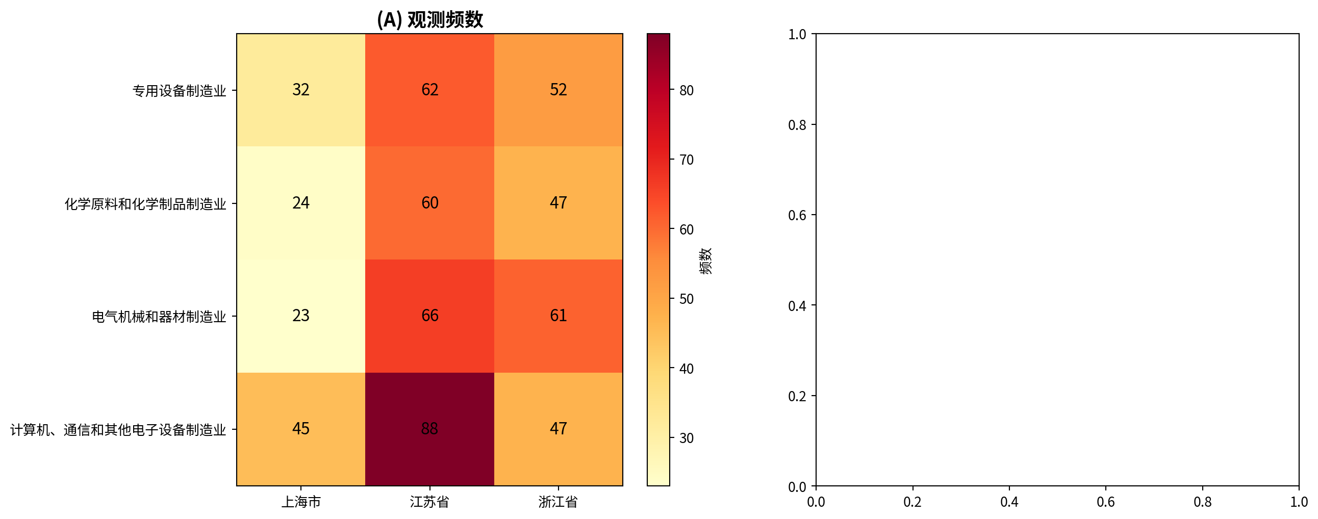
左子图(观测频数)绘制完毕。下面绘制右子图(标准化残差热图),其中|残差|>2的格子表示观测值显著偏离独立性假设下的期望值。
The left subplot (observed frequencies) has been drawn. Below we draw the right subplot (standardized residuals heatmap), where cells with |residual| > 2 indicate that observed values deviate significantly from the expected values under the independence assumption.
# --- 右图: 标准化残差热图 ---
# --- Right panel: standardized residuals heatmap ---
heatmap_image_2 = matplot_axes_array[1].imshow(                                   # 用红蓝配色渲染残差
    # Render residuals with a red-blue color scheme
    heatmap_std_residuals, cmap='RdBu_r', vmin=-3, vmax=3, aspect='auto'          # 对称色阶[-3, 3]
    # Symmetric color scale [-3, 3]
)
matplot_axes_array[1].set_xticks(np.arange(len(heatmap_col_labels)))              # x轴刻度
# x-axis ticks
matplot_axes_array[1].set_yticks(np.arange(len(heatmap_row_labels)))              # y轴刻度
# y-axis ticks
matplot_axes_array[1].set_xticklabels(heatmap_col_labels)                         # 省份标签
# Province labels
matplot_axes_array[1].set_yticklabels(heatmap_row_labels)                         # 行业标签
# Industry labels
matplot_axes_array[1].set_title(                                                  # 子图标题
    # Subplot title
    '(B) 标准化残差 (|残差|>2为显著)', fontsize=14, fontweight='bold'          # 标题文本及样式
    # Title text and style
)

for row_index_i in range(len(heatmap_row_labels)):                                # 在每个格子中标注残差值
    # Annotate each cell with its residual value
    for col_index_j in range(len(heatmap_col_labels)):                             # 遍历列索引
        # Iterate over column indices
        cell_text_color = (                                                        # |残差|≥2用白字突出显示
            # Use white text to highlight |residual| ≥ 2
            'black' if abs(heatmap_std_residuals[row_index_i, col_index_j]) < 2    # 残差绝对值<2用黑字
            # Black text if absolute residual < 2
            else 'white'                                                           # 残差绝对值≥2用白字突出
            # White text if absolute residual ≥ 2 for emphasis
        )
        matplot_axes_array[1].text(                                                # 在指定位置添加文本标注
            # Add text annotation at the specified position
            col_index_j, row_index_i,                                              # 文本位置坐标(x, y)
            # Text position coordinates (x, y)
            f'{heatmap_std_residuals[row_index_i, col_index_j]:.1f}',              # 标准化残差值保留1位小数
            # Standardized residual value rounded to 1 decimal place
            ha='center', va='center', color=cell_text_color,                       # 居中对齐,根据残差大小设置颜色
            # Center alignment, color set based on residual magnitude
            fontsize=11, fontweight='bold'                                         # 字体11号加粗
            # Font size 11, bold
        )

plt.colorbar(heatmap_image_2, ax=matplot_axes_array[1], label='标准化残差')        # 添加颜色条
# Add a colorbar

plt.tight_layout()                                                                 # 自动调整间距
# Automatically adjust spacing
plt.show()                                                                         # 显示热图
# Display the heatmap
<Figure size 672x480 with 0 Axes>图 6.1 的左图(A面板)为观测频数热图,右图(B面板)为标准化残差热图。从频数热图可以看到,江苏省在各行业的公司数量普遍较多(颜色较深),尤其是计算机通信行业(88家);上海在计算机通信行业也有相对集中(45家)。残差热图中,整体色调偏淡,没有出现深红或深蓝的格子——这意味着没有任何行业-地区组合呈现出令人惊讶的异常频数。最引人注目的是计算机通信×浙江的浅蓝色(残差 -1.84)和电气机械×上海的浅蓝色(残差 -1.38),但它们均未超过 \(|2|\) 的显著阈值。这一可视化结果从直觉上验证了前文卡方检验”不能拒绝独立性”的统计结论。
The left panel (Panel A) of 图 6.1 shows the observed frequency heatmap, and the right panel (Panel B) shows the standardized residuals heatmap. From the frequency heatmap, we can see that Jiangsu Province generally has more companies in each industry (darker colors), especially in the computer and telecommunications industry (88 firms); Shanghai also shows relative concentration in the computer and telecommunications industry (45 firms). In the residuals heatmap, the overall color tone is muted, with no deep red or deep blue cells — this means no industry–region combination exhibits a surprisingly anomalous frequency. The most notable cells are the light blue for computer & telecommunications × Zhejiang (residual −1.84) and electrical machinery × Shanghai (residual −1.38), but neither exceeds the significance threshold of \(|2|\). This visualization intuitively corroborates the earlier chi-square test’s statistical conclusion that “we cannot reject independence.” ## 其他类型的卡方检验 (Other Types of Chi-Square Tests) {#sec-other-chisq-tests}
6.5.5 齐性检验(Homogeneity Test)
检验不同群体在某个分类变量的分布是否相同。
Tests whether different populations have the same distribution for a categorical variable.
与独立性检验的区别:
- 独立性检验: 从一个总体中抽样,考察两个变量的关联
- 齐性检验: 从多个总体中分别抽样,比较它们的分布是否一致
Difference from the Independence Test:
- Independence test: Sampling from one population to examine the association between two variables
- Homogeneity test: Sampling separately from multiple populations to compare whether their distributions are the same
计算方法: 卡方统计量计算公式相同,但抽样方式不同
Computation method: The chi-square statistic formula is the same, but the sampling design differs.
6.5.6 McNemar检验(配对卡方检验) (McNemar Test / Paired Chi-Square Test)
适用于配对二分类数据的检验,例如:
- 同一组对象在干预前后的状态变化
- 两种诊断方法对同一组样本的诊断结果比较
Applicable to tests on paired binary data, for example:
- Changes in status of the same group of subjects before and after an intervention
- Comparing diagnostic results of two diagnostic methods on the same set of samples
检验统计量:
Test statistic:
McNemar 检验的统计量如 式 6.4 所示:
The McNemar test statistic is shown in 式 6.4:
\[ \chi^2 = \frac{(b - c)^2}{b + c} \tag{6.4}\]
其中 \(b\) 和 \(c\) 是不一致的配对数。
where \(b\) and \(c\) are the number of discordant pairs.
校正版本 (适用于小样本):
Corrected version (for small samples):
\[ \chi^2_{corr} = \frac{(|b - c| - 1)^2}{b + c} \]
6.6 Fisher精确检验 (Fisher’s Exact Test)
6.6.1 适用场景 (Applicable Scenarios)
当样本量很小(理论频数 \(< 5\)),卡方检验的近似不准确时,应使用Fisher精确检验。
When the sample size is small (expected frequency \(< 5\)) and the chi-square approximation becomes inaccurate, Fisher’s exact test should be used.
原理: 基于超几何分布,计算在边际和固定的条件下,获得当前观测列联表的精确概率。
Principle: Based on the hypergeometric distribution, it calculates the exact probability of obtaining the observed contingency table given fixed marginal totals.
优点:
- 精确,不依赖大样本近似
- 适用于 \(2 \times 2\) 表
Advantages:
- Exact; does not rely on large-sample approximation
- Suitable for \(2 \times 2\) tables
缺点:
- 计算量大(尤其当样本量大时)
- 难以扩展到大表
Disadvantages:
- Computationally intensive (especially with large sample sizes)
- Difficult to extend to larger tables
6.6.2 案例:小样本案例 (Case Study: Small Sample Example)
什么是小样本下的模型比较?
What is model comparison under small samples?
在金融风控实践中,新模型上线前通常需要小规模试点。由于试点期间的样本量往往很小(如仅有50笔异常交易),常规的卡方检验可能因为期望频数过低而失效。这时,我们需要一种在小样本条件下仍然精确有效的检验方法。
In financial risk management practice, a small-scale pilot is usually required before deploying a new model. Because the sample size during the pilot phase is often very small (e.g., only 50 abnormal transactions), the conventional chi-square test may fail due to low expected frequencies. In such cases, we need a test that remains exact and valid under small-sample conditions.
Fisher精确检验通过枚举所有可能的列联表排列,计算精确的p值,不依赖大样本近似,因此特别适合小样本场景。下面是一个典型的应用场景:某长三角地区证券公司的风控部门正在评估新旧两套风控预警模型,由于试点期间仅抽取了50笔异常交易进行人工复核,样本量较小,因此采用Fisher精确检验比较两套模型的预警判断是否存在显著差异,结果如 表 6.3 所示。
Fisher’s exact test enumerates all possible arrangements of the contingency table and computes an exact p-value without relying on large-sample approximation, making it particularly suitable for small-sample scenarios. Below is a typical application: the risk management department of a securities company in the Yangtze River Delta region is evaluating two risk-alert models (old vs. new). Since only 50 abnormal transactions were sampled for manual review during the pilot, the sample size is small, so Fisher’s exact test is used to compare whether the alert decisions of the two models differ significantly. The results are shown in 表 6.3.
# ========== 导入所需库 ==========
# ========== Import required libraries ==========
from scipy.stats import fisher_exact          # Fisher精确检验函数
# Fisher's exact test function
import numpy as np                             # 数值计算库
# Numerical computing library

# ========== 第1步:构建2×2观测列联表 ==========
# ========== Step 1: Construct the 2×2 observed contingency table ==========
# 场景:某证券公司对新旧两套风控预警模型进行对比评估
# Scenario: A securities company compares old and new risk-alert models
# 行表示旧模型预警结果,列表示新模型预警结果
# Rows represent old model alert results; columns represent new model alert results
observed_alert_matrix = np.array([                                               # 构建2×2观测列联表矩阵
# Construct the 2×2 observed contingency table matrix
    [15, 5],                                   # 旧模型预警: 新模型也预警15笔, 新模型未预警5笔
    # Old model alerted: new model also alerted 15, new model did not alert 5
    [10, 20]                                   # 旧模型未预警: 新模型预警10笔, 新模型也未预警20笔
    # Old model did not alert: new model alerted 10, new model also did not alert 20
])

# ========== 第2步:打印观测列联表 ==========
# ========== Step 2: Print the observed contingency table ==========
print('=' * 60)                                # 分隔线
# Separator line
print('Fisher精确检验:风控预警模型比较')         # 标题
# Title: Fisher's exact test: risk-alert model comparison
print('=' * 60)                                # 分隔线
# Separator line

print('\n观测列联表:')                          # 表头
# Header: Observed contingency table
print('                新模型预警  新模型未预警  合计')                # 输出列标题
# Column headers: New model alerted / New model not alerted / Total
print('-' * 50)                                # 分隔线
# Separator line
alert_row_labels = ['旧模型预警', '旧模型未预警']      # 行标签(旧模型预警结果)
# Row labels (old model alert results)
for ind_i, row_data in enumerate(observed_alert_matrix):    # 逐行打印
# Iterate and print each row
    print(f'{alert_row_labels[ind_i]:10s}  {row_data[0]:10d}  {row_data[1]:10d}  {row_data.sum():5d}')  # 输出每行观测值及行合计
    # Print observed values and row total for each row

alert_col_sums_array = observed_alert_matrix.sum(axis=0)    # 列合计
# Column totals
print(f'{"合计":10s}  {alert_col_sums_array[0]:10d}  {alert_col_sums_array[1]:10d}  {alert_col_sums_array.sum():5d}')  # 输出合计行
# Print totals row
============================================================
Fisher精确检验:风控预警模型比较
============================================================
观测列联表:
新模型预警 新模型未预警 合计
--------------------------------------------------
旧模型预警 15 5 20
旧模型未预警 10 20 30
合计 25 25 50上述代码输出了一个 \(2 \times 2\) 观测列联表,总样本量为50笔交易。其中,旧模型预警的20笔中,新模型也预警了15笔(一致)、但有5笔新模型未预警(遗漏);旧模型未预警的30笔中,新模型预警了10笔(新增发现)、20笔两套模型均未预警(一致)。从边际合计看,新模型共预警25笔、未预警25笔,而旧模型预警20笔、未预警30笔,新模型整体预警率更高。要严格检验两套模型的预警结果是否存在显著差异,我们需要使用Fisher精确检验。
The code above outputs a \(2 \times 2\) observed contingency table with a total sample size of 50 transactions. Among the 20 transactions flagged by the old model, the new model also flagged 15 (agreement) but missed 5 (omission). Among the 30 transactions not flagged by the old model, the new model flagged 10 (new discoveries) while both models agreed on 20 as non-alerts. Looking at the marginal totals, the new model flagged 25 transactions in total versus the old model’s 20, indicating a higher overall alert rate. To rigorously test whether the alert outcomes of the two models differ significantly, we need to use Fisher’s exact test.
观测列联表输出完毕。下面执行Fisher精确检验。
The observed contingency table has been printed. Now we proceed to perform Fisher’s exact test.
# ========== 第3步:执行Fisher精确检验 ==========
# ========== Step 3: Perform Fisher's exact test ==========
fisher_odds_ratio, fisher_calculated_p_value = fisher_exact(       # 双侧检验
# Two-sided test
    observed_alert_matrix, alternative='two-sided'                  # 传入2×2矩阵执行Fisher精确检验
    # Pass the 2×2 matrix to perform Fisher's exact test
)

print(f'\nFisher精确检验结果:')                  # 输出检验结果
# Print test results
print(f'  比值比 (Odds Ratio): {fisher_odds_ratio:.3f}')          # 比值比
# Odds ratio
print(f'  p值 (双侧): {fisher_calculated_p_value:.6f}')           # 精确p值
# Exact p-value (two-sided)
Fisher精确检验结果:
  比值比 (Odds Ratio): 6.000
  p值 (双侧): 0.008579
Fisher精确检验结果显示:比值比(Odds Ratio)为6.000,双侧精确p值为0.008579。OR=6.000意味着,在旧模型预警的分组中,新模型也预警的比值是新模型未预警比值的6倍。换言之,当旧模型发出预警时,新模型同样发出预警的可能性远大于不发出预警的可能性,两套模型在”高风险”区域表现出较强的一致性,但在”低风险”区域存在显著分歧(新模型新增了10笔旧模型未识别的预警)。
The Fisher’s exact test results show: the odds ratio (OR) is 6.000 and the two-sided exact p-value is 0.008579. An OR of 6.000 means that within the group flagged by the old model, the odds of the new model also flagging is 6 times the odds of it not flagging. In other words, when the old model issues an alert, it is far more likely that the new model also issues an alert than not, indicating strong agreement between the two models in the “high-risk” zone. However, there is a significant divergence in the “low-risk” zone (the new model newly flagged 10 transactions that the old model missed).
Fisher精确检验计算完成。下面给出统计结论,并与Yates校正卡方检验对比。
Fisher’s exact test computation is complete. Below we present the statistical conclusion and compare it with the Yates-corrected chi-square test.
# ========== 第4步:给出统计结论 ==========
# ========== Step 4: Present the statistical conclusion ==========
print(f'\n结论 (α=0.05):')                      # 显著性水平α=0.05
# Conclusion at significance level α=0.05
if fisher_calculated_p_value < 0.05:            # p值小于α则拒绝原假设
# If p-value < α, reject the null hypothesis
    print(f'  拒绝H0 (p={fisher_calculated_p_value:.6f} < 0.05)')             # 输出拒绝结论
    # Print rejection conclusion
    print(f'  两套风控模型的预警结果存在显著差异')                        # 说明模型差异显著
    # The alert outcomes of the two risk models differ significantly
    print(f'  比值比{fisher_odds_ratio:.3f}表明:')                        # 提示比值比含义
    # The odds ratio indicates:
    if fisher_odds_ratio > 1:                   # OR>1说明新模型预警更多
    # OR > 1 means the new model alerts more
        print(f'    - 新模型倾向于发出更多预警信号')                      # 新模型更敏感
        # The new model tends to issue more alert signals
    else:                                       # OR<1说明新模型预警更少
    # OR < 1 means the new model alerts less
        print(f'    - 新模型倾向于发出更少预警信号')                      # 新模型更保守
        # The new model tends to issue fewer alert signals
else:                                           # p值≥α则不能拒绝原假设
# If p-value >= α, fail to reject the null hypothesis
    print(f'  不能拒绝H0 (p={fisher_calculated_p_value:.6f} >= 0.05)')     # 输出不拒绝结论
    # Print fail-to-reject conclusion
    print(f'  没有证据表明两套风控模型的预警存在差异')                # 无显著差异
    # No evidence that the two risk models' alerts differ

# ========== 第5步:与Yates校正卡方检验对比 ==========
# ========== Step 5: Compare with Yates-corrected chi-square test ==========
from scipy.stats import chi2_contingency        # 导入卡方检验函数
# Import the chi-square test function
yates_chi2_statistic, yates_p_value, yates_dof, _ = chi2_contingency(   # Yates连续性校正
# Yates continuity correction
    observed_alert_matrix, correction=True                              # 开启校正以适应小样本
    # Enable correction for small samples
)

print(f'\n对比: Yates校正卡方检验')              # 输出对比结果
# Comparison: Yates-corrected chi-square test
print(f'  卡方统计量: {yates_chi2_statistic:.4f}')                      # 卡方统计量
# Chi-square statistic
print(f'  p值: {yates_p_value:.6f}')                                    # 近似p值
# Approximate p-value
print(f'  注: 当样本量较小时,Fisher检验更准确')                           # 方法适用性说明
# Note: When sample size is small, Fisher's test is more accurate
结论 (α=0.05):
  拒绝H0 (p=0.008579 < 0.05)
  两套风控模型的预警结果存在显著差异
  比值比6.000表明:
    - 新模型倾向于发出更多预警信号

对比: Yates校正卡方检验
  卡方统计量: 6.7500
  p值: 0.009375
  注: 当样本量较小时,Fisher检验更准确
上述代码的运行结果分为两部分。第一部分是Fisher精确检验的统计结论:在 \(\alpha = 0.05\) 水平下,p值=0.008579 < 0.05,拒绝原假设 \(H_0\)(两套模型的预警结果无差异),即两套风控模型的预警结果存在统计上的显著差异。比值比OR=6.000(大于1)表明新模型倾向于发出更多预警信号,说明新模型的风险识别灵敏度更高。
The results above consist of two parts. The first part is the statistical conclusion from Fisher’s exact test: at \(\alpha = 0.05\), the p-value = 0.008579 < 0.05, so we reject the null hypothesis \(H_0\) (that the alert outcomes of the two models are the same). This means the alert outcomes of the two risk models are statistically significantly different. The odds ratio OR = 6.000 (greater than 1) indicates that the new model tends to issue more alerts, suggesting higher risk-detection sensitivity.
第二部分是与Yates校正卡方检验的对比:Yates校正 \(\chi^2 = 6.7500\),对应p值为0.009375,同样显著。两种方法结论一致(均拒绝 \(H_0\)),但Fisher精确检验的p值(0.008579)比Yates校正(0.009375)略低。在总样本量仅50笔、且部分格子期望频数较小的条件下,Fisher精确检验基于精确概率分布计算,不依赖大样本渐近近似,因此结果更为可靠。这验证了”当样本量较小或期望频数低于5时,应优先使用Fisher精确检验”的方法论原则。
The second part compares with the Yates-corrected chi-square test: Yates-corrected \(\chi^2 = 6.7500\) with a corresponding p-value of 0.009375, which is also significant. Both methods reach the same conclusion (both reject \(H_0\)), but Fisher’s exact test yields a slightly lower p-value (0.008579) than the Yates correction (0.009375). With only 50 transactions and some cells having small expected frequencies, Fisher’s exact test computes based on exact probability distributions without relying on large-sample asymptotic approximation, making the result more reliable. This validates the methodological principle that “when the sample size is small or expected frequencies fall below 5, Fisher’s exact test should be preferred.”
6.6.3 启发式思考题 (Heuristic Problems)
1. 彩票随机性检验 (The Lottery Randomness Test)
许多老彩民坚信彩票有”走势图”。
任务:获取中国福利彩票”双色球”最近100期的红球开奖数据(1-33号)。
统计每个号码出现的频率。
使用拟合优度检验:它们是否服从均匀分布?
如果 P < 0.05,你会怎么做?(提示:样本量才100期×6球=600个号,33个类别,期望频数约18,检验是有效的。如果显著,可能意味着…机器偏差?)
Many veteran lottery players firmly believe that lottery numbers follow “trend charts.”
Task: Obtain the red ball draw data (numbers 1–33) from the most recent 100 draws of China’s Welfare Lottery “Double Color Ball.”
Count the frequency of each number.
Use the goodness-of-fit test: Do they follow a uniform distribution?
If P < 0.05, what would you do? (Hint: The sample size is only 100 draws × 6 balls = 600 numbers, 33 categories, expected frequency ~18—the test is valid. If significant, it might mean… machine bias?)
# ========== 导入所需库 ==========
# ========== Import required libraries ==========
import numpy as np                             # 数值计算库
# Numerical computing library
from scipy.stats import chisquare             # 卡方拟合优度检验
# Chi-square goodness-of-fit test
import matplotlib.pyplot as plt                # 绘图库
# Plotting library

# ========== 第1步:设定模拟参数 ==========
# ========== Step 1: Set simulation parameters ==========
# 注:此处使用模拟数据演示统计检验方法的应用过程
# Note: Simulated data is used here to demonstrate the application of the statistical test
np.random.seed(42)                             # 固定随机种子,保证可复现
# Fix random seed for reproducibility
total_lottery_draws_count = 100                # 模拟100期开奖
# Simulate 100 lottery draws
red_balls_per_draw_count = 6                   # 每期抽取6个红球
# 6 red balls per draw
max_red_ball_number = 33                       # 红球号码范围1-33
# Red ball numbers range from 1 to 33

# ========== 第2步:模拟每期开奖数据 ==========
# ========== Step 2: Simulate draw data for each period ==========
all_drawn_red_balls_list = []                  # 存储所有期的红球号码
# Store all drawn red ball numbers
for draw_index in range(total_lottery_draws_count):              # 逐期模拟
# Simulate each draw
    single_draw_balls = np.random.choice(                        # 从1-33中不放回抽取6个
    # Sample 6 without replacement from 1–33
        range(1, max_red_ball_number + 1),                        # 号码范围1刳33
        # Number range 1 to 33
        size=red_balls_per_draw_count, replace=False              # 抽取6个,不放回
        # Draw 6, without replacement
    )
    all_drawn_red_balls_list.extend(single_draw_balls)           # 追加到总列表
    # Append to the master list

all_drawn_red_balls_array = np.array(all_drawn_red_balls_list)   # 转为NumPy数组
# Convert to NumPy array

# ========== 第3步:统计每个号码的观测频数 ==========
# ========== Step 3: Count the observed frequency of each number ==========
observed_ball_frequencies = np.zeros(max_red_ball_number)        # 初始化33个号码的频数
# Initialize frequency array for 33 numbers
for ball_number in range(1, max_red_ball_number + 1):            # 遍历每个号码
# Iterate over each number
    observed_ball_frequencies[ball_number - 1] = np.sum(         # 统计该号码出现次数
    # Count occurrences of this number
        all_drawn_red_balls_array == ball_number                  # 比较数组中等于当前号码的元素
        # Compare array elements equal to the current number
    )
彩票开奖模拟和号码频数统计完成。下面计算均匀分布下的理论频数,并执行卡方拟合优度检验。
Lottery draw simulation and number frequency counting are complete. Next, we compute the theoretical frequencies under a uniform distribution and perform the chi-square goodness-of-fit test.
# ========== 第4步:计算均匀分布下的理论频数 ==========
# ========== Step 4: Calculate theoretical frequencies under uniform distribution ==========
# 每期抽6个,共100期,总共600个球;均匀分布下每个号码期望 = 600/33
# 6 balls per draw × 100 draws = 600 balls total; expected frequency per number under uniform = 600/33
total_balls_drawn_count = total_lottery_draws_count * red_balls_per_draw_count   # 总球数600
# Total number of balls: 600
uniform_expected_frequency = total_balls_drawn_count / max_red_ball_number       # 每号期望≈18.18
# Expected frequency per number ≈ 18.18
expected_ball_frequencies = np.full(max_red_ball_number, uniform_expected_frequency)  # 33个相同期望值
# Array of 33 identical expected values

# ========== 第5步:执行卡方拟合优度检验 ==========
# ========== Step 5: Perform chi-square goodness-of-fit test ==========
chi2_lottery_statistic, lottery_p_value = chisquare(             # H0: 各号码服从均匀分布
# H0: Each number follows a uniform distribution
    observed_ball_frequencies, f_exp=expected_ball_frequencies     # 传入观测与期望频数
    # Pass observed and expected frequencies
)

print('=' * 60)                                                  # 分隔线
# Separator line
print('彩票随机性检验:双色球红球号码拟合优度检验')               # 标题
# Title: Lottery randomness test: Double Color Ball red ball goodness-of-fit test
print('=' * 60)                                                  # 分隔线
# Separator line
print(f'总开奖期数: {total_lottery_draws_count}')                # 期数
# Total number of draws
print(f'总红球个数: {total_balls_drawn_count}')                  # 总球数
# Total number of red balls
print(f'每个号码的理论频数 (均匀分布): {uniform_expected_frequency:.2f}')  # 期望频数
# Theoretical frequency per number (uniform distribution)
print(f'\n卡方统计量: {chi2_lottery_statistic:.4f}')             # χ²值
# Chi-square statistic
print(f'自由度: {max_red_ball_number - 1}')                      # df = 33-1 = 32
# Degrees of freedom = 33 - 1 = 32
print(f'p值: {lottery_p_value:.4f}')                             # p值
# p-value

if lottery_p_value < 0.05:                                       # 显著性判断
# Significance assessment
    print('结论: 拒绝均匀分布假设 → 号码出现频率存在显著偏差')            # 拒绝H0的结论
    # Conclusion: Reject the uniform distribution hypothesis → significant deviation in number frequencies
else:                                                            # p值≥α时
# When p-value >= α
    print('结论: 不能拒绝均匀分布假设 → 没有证据表明开奖不随机')       # 不拒绝H0的结论
    # Conclusion: Fail to reject the uniform distribution hypothesis → no evidence that draws are non-random
============================================================
彩票随机性检验:双色球红球号码拟合优度检验
============================================================
总开奖期数: 100
总红球个数: 600
每个号码的理论频数 (均匀分布): 18.18
卡方统计量: 36.5700
自由度: 32
p值: 0.2648
结论: 不能拒绝均匀分布假设 → 没有证据表明开奖不随机卡方拟合优度检验结果显示:在模拟的100期双色球开奖中,共产生600个红球号码,每个号码(1-33号)在均匀分布假设下的期望频数为18.18次。检验统计量 \(\chi^2 = 36.5700\),自由度 \(df = 32\),p值=0.2648。由于p值远大于0.05,我们不能拒绝均匀分布的原假设,即没有统计证据表明某些号码出现的频率高于其他号码。这一结果符合预期——模拟数据本就来自均匀分布的随机抽样过程。在实际应用中,这意味着:即便某些号码在短期内”扎堆”出现,只要样本量合理(此处600次观测、33个类别、每个类别期望频数约18),拟合优度检验就能有效区分随机波动和系统性偏差。所谓”彩票走势图”在统计学检验面前缺乏依据。
The chi-square goodness-of-fit test results show: in the simulated 100 draws of Double Color Ball, a total of 600 red ball numbers were generated. Under the uniform distribution hypothesis, the expected frequency for each number (1–33) is 18.18. The test statistic \(\chi^2 = 36.5700\), degrees of freedom \(df = 32\), and p-value = 0.2648. Since the p-value is far greater than 0.05, we fail to reject the null hypothesis of uniform distribution—there is no statistical evidence that some numbers appear more frequently than others. This result is expected, as the simulated data is generated from a uniformly random sampling process. In practice, this means: even if some numbers appear to “cluster” in the short term, as long as the sample size is reasonable (here, 600 observations, 33 categories, expected frequency ~18 per category), the goodness-of-fit test can effectively distinguish random fluctuation from systematic bias. The so-called “lottery trend charts” lack any statistical basis.
基于卡方拟合优度检验结果,我们绘制柱状图可视化各号码的观测频数与均匀分布期望频数的对比:
Based on the chi-square goodness-of-fit test results, we plot a bar chart to visualize the comparison between the observed frequency of each number and the expected frequency under a uniform distribution:
# ========== 第6步:可视化——柱状图 + 均匀分布参考线 ==========
# ========== Step 6: Visualization — Bar chart + uniform distribution reference line ==========
matplot_figure, matplot_axes = plt.subplots(figsize=(12, 5))     # 创建画布
# Create figure canvas
ball_number_labels = np.arange(1, max_red_ball_number + 1)       # x轴标签1-33
# X-axis labels from 1 to 33

bar_colors_list = [                                               # 高于期望值用红色标记
# Mark those above expected with red
    '#E3120B' if freq > uniform_expected_frequency else '#2C3E50' # 超出期望为红色,否则为深蓝
    # Red if above expected, dark blue otherwise
    for freq in observed_ball_frequencies                          # 遍历每个号码的观测频数
    # Iterate over observed frequency of each number
]
matplot_axes.bar(                                                 # 绘制柱状图
# Plot bar chart
    ball_number_labels, observed_ball_frequencies,                 # x轴为号码,y轴为频数
    # x-axis: number, y-axis: frequency
    color=bar_colors_list, alpha=0.8                              # 按颜色列表填充,透明度0.8
    # Fill by color list, transparency 0.8
)

matplot_axes.axhline(                                             # 均匀分布参考线
# Uniform distribution reference line
    y=uniform_expected_frequency, color='orange', linestyle='--', # 橘色虚线表示期望值
    # Orange dashed line indicates expected value
    linewidth=2, label=f'均匀分布期望频数 = {uniform_expected_frequency:.1f}'  # 图例标签
    # Legend label
)

matplot_axes.set_xlabel('红球号码', fontsize=12)                    # x轴标签
# X-axis label: Red ball number
matplot_axes.set_ylabel('出现次数', fontsize=12)                    # y轴标签
# Y-axis label: Occurrences
matplot_axes.set_title(                                            # 图标题(含检验统计量)
# Figure title (including test statistics)
    f'双色球红球号码频数分布 (模拟{total_lottery_draws_count}期, '         # 标题第一行
    # Title line 1: Red ball frequency distribution (simulated N draws)
    f'χ²={chi2_lottery_statistic:.2f}, p={lottery_p_value:.3f})',              # 标题第二行:检验统计量
    # Title line 2: test statistics
    fontsize=13                                                    # 字号大小13
    # Font size 13
)
matplot_axes.set_xticks(ball_number_labels)                        # 设置x轴刻度
# Set x-axis ticks
matplot_axes.legend()                                              # 显示图例
# Show legend
plt.tight_layout()                                                 # 自动调整间距
# Auto-adjust spacing
plt.show()                                                         # 显示柱状图
# Display bar chart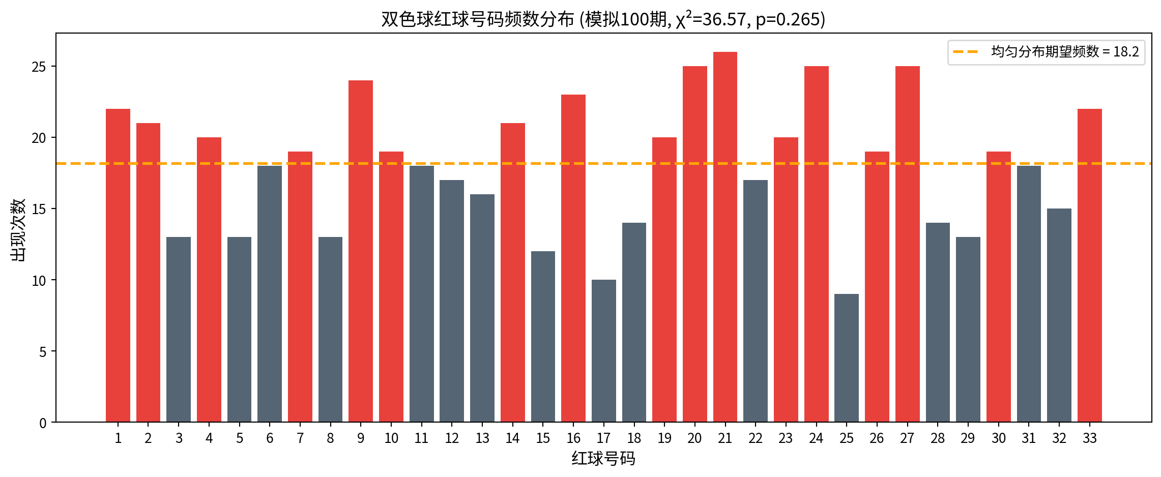
图 6.2 展示了33个红球号码各自的观测频数柱状图。其中深蓝色柱形表示低于均匀期望频数的号码,红色柱形表示高于期望频数的号码,橘色水平虚线标注了均匀分布期望频数(约18.2次)。从图中可以看到,各号码的观测频数在期望值上下自然波动,没有任何号码出现极端的高频或低频偏离。这种围绕期望值的随机波动模式,与p值=0.265(远未达到0.05显著性水平)的检验结论完全一致,直观地说明了”在随机抽样过程中,短期频率偏差属于正常的统计噪声”。
图 6.2 displays a bar chart of the observed frequency for each of the 33 red ball numbers. Dark blue bars indicate numbers below the uniform expected frequency, red bars indicate those above, and the orange horizontal dashed line marks the uniform distribution’s expected frequency (~18.2). As seen in the figure, the observed frequencies fluctuate naturally around the expected value, with no number exhibiting an extreme high or low deviation. This pattern of random fluctuation around the expected value is fully consistent with the test conclusion of p = 0.265 (far from the 0.05 significance level), intuitively illustrating that “in a random sampling process, short-term frequency deviations represent normal statistical noise.”
2. 星座与成功 (Zodiac and Success)
经常有文章说”某个星座最容易出亿万富翁”。
任务:收集福布斯中国富豪榜前100名的出生日期,确定其星座。
统计12星座的频数。
各种星座的人口基数假设是相等的(或者根据出生月份天数微调)。
进行卡方检验。结果显著吗?
警示:如果你的 P值是 0.04,你会以此为标题发表文章吗?(记得我们在第5章讨论的 P-Hacking 和多重比较问题吗?)
There are often articles claiming “a certain zodiac sign is most likely to produce billionaires.”
Task: Collect the birth dates of the top 100 on the Forbes China Rich List and determine their zodiac signs.
Count the frequency of each of the 12 zodiac signs.
Assume the population base for each zodiac sign is equal (or adjust slightly based on the number of days in each birth month).
Perform a chi-square test. Is the result significant?
Warning: If your p-value is 0.04, would you publish an article with this as the headline? (Remember the P-Hacking and multiple comparison issues we discussed in Chapter 5?)
# ========== 导入所需库 ==========
# ========== Import required libraries ==========
import numpy as np                             # 数值计算库
# Numerical computing library
from scipy.stats import chisquare             # 卡方拟合优度检验
# Chi-square goodness-of-fit test
import matplotlib.pyplot as plt                # 绘图库
# Plotting library

# ========== 第1步:定义12星座及对应天数 ==========
# ========== Step 1: Define the 12 zodiac signs and their corresponding days ==========
# 注:此处使用模拟数据来演示如何用卡方检验评估"星座决定成功"这一伪科学命题
# Note: Simulated data is used here to demonstrate how to evaluate the pseudoscientific claim "zodiac determines success" using a chi-square test
np.random.seed(2024)                           # 固定随机种子
# Fix random seed

zodiac_names_list = [                          # 12星座名称
# Names of the 12 zodiac signs
    '水瓶座', '双鱼座', '白羊座', '金牛座', '双子座', '巨蟹座',
    '狮子座', '处女座', '天秤座', '天蝎座', '射手座', '摩羯座'
]
zodiac_days_array = np.array([                 # 每个星座对应的天数(近似值)
# Number of days for each zodiac sign (approximate)
    30, 29, 31, 30, 31, 30,                   # 水瓶-巨蟹
    # Aquarius–Cancer
    31, 31, 30, 30, 30, 31                     # 狮子-摩羯
    # Leo–Capricorn
])
12星座名称与天数定义完毕。下面按天数计算理论比例并模拟富豪星座分布。
The 12 zodiac sign names and their day counts have been defined. Next, we calculate the theoretical proportions based on days and simulate the zodiac distribution of billionaires.
# ========== 第2步:计算理论比例(按天数加权) ==========
# ========== Step 2: Calculate theoretical proportions (weighted by days) ==========
zodiac_theoretical_proportions = (              # 按天数占比作为理论概率
# Use day proportions as theoretical probabilities
    zodiac_days_array / zodiac_days_array.sum()  # 各星座天数除以总天数
    # Each sign's days divided by total days
)

# ========== 第3步:模拟100位富豪的星座分布 ==========
# ========== Step 3: Simulate the zodiac distribution of 100 billionaires ==========
billionaire_sample_size = 100                   # 模拟100位富豪
# Simulate 100 billionaires
zodiac_expected_frequencies = (                 # 各星座的理论期望频数
# Theoretical expected frequency for each zodiac sign
    zodiac_theoretical_proportions * billionaire_sample_size  # 理论概率×样本量
    # Theoretical probability × sample size
)

zodiac_observed_frequencies = np.random.multinomial(   # 按理论比例多项式抽样
# Multinomial sampling according to theoretical proportions
    billionaire_sample_size, zodiac_theoretical_proportions  # 总数和各类概率
    # Total count and category probabilities
)
富豪星座分布模拟完成。下面执行卡方拟合优度检验,判断星座分布是否与理论比例存在显著差异。
Billionaire zodiac distribution simulation is complete. Next, we perform the chi-square goodness-of-fit test to determine whether the zodiac distribution differs significantly from the theoretical proportions.
# ========== 第4步:执行卡方拟合优度检验 ==========
# ========== Step 4: Perform chi-square goodness-of-fit test ==========
chi2_zodiac_statistic, zodiac_p_value = chisquare(     # H0: 富豪星座服从理论分布
# H0: Billionaire zodiac signs follow the theoretical distribution
    zodiac_observed_frequencies, f_exp=zodiac_expected_frequencies  # 观测频数与期望频数
    # Observed frequencies and expected frequencies
)

print('=' * 60)                                         # 分隔线
# Separator line
print('星座与成功:富豪星座分布的卡方检验')               # 标题
# Title: Zodiac and Success: Chi-square test on billionaire zodiac distribution
print('=' * 60)                                         # 分隔线
# Separator line
print(f'样本量: {billionaire_sample_size} 位模拟富豪')   # 输出样本量
# Sample size: N simulated billionaires

print(f'\n星座      观测频数  理论频数  差异')            # 表头
# Header: Zodiac / Observed / Expected / Difference
print('-' * 45)                                         # 分隔线
# Separator line
for idx in range(12):                                   # 逐星座打印
# Print for each zodiac sign
    difference_value = (                                 # 计算观测与理论的差异
    # Calculate difference between observed and expected
        zodiac_observed_frequencies[idx] - zodiac_expected_frequencies[idx]  # 观测-期望
        # Observed minus expected
    )
    print(f'{zodiac_names_list[idx]:5s}  {zodiac_observed_frequencies[idx]:8d}  '  # 星座名+观测
    # Zodiac name + observed count
          f'{zodiac_expected_frequencies[idx]:8.1f}  {difference_value:+6.1f}')    # 期望+差异
    # Expected + difference

print(f'\n卡方统计量: {chi2_zodiac_statistic:.4f}')      # χ²值
# Chi-square statistic
print(f'自由度: {12 - 1}')                               # df = 12-1 = 11
# Degrees of freedom = 12 - 1 = 11
print(f'p值: {zodiac_p_value:.4f}')                      # p值
# p-value
============================================================
星座与成功:富豪星座分布的卡方检验
============================================================
样本量: 100 位模拟富豪
星座 观测频数 理论频数 差异
---------------------------------------------
水瓶座 9 8.2 +0.8
双鱼座 9 8.0 +1.0
白羊座 6 8.5 -2.5
金牛座 4 8.2 -4.2
双子座 7 8.5 -1.5
巨蟹座 6 8.2 -2.2
狮子座 12 8.5 +3.5
处女座 11 8.5 +2.5
天秤座 9 8.2 +0.8
天蝎座 9 8.2 +0.8
射手座 5 8.2 -3.2
摩羯座 13 8.5 +4.5
卡方统计量: 9.9342
自由度: 11
p值: 0.5363运行结果展示了100位模拟富豪在12个星座上的分布情况。各星座的理论期望频数根据每个星座跨越的天数进行加权计算(例如,31天的星座期望频数为8.5,29天的双鱼座仅8.0)。观测频数与理论频数的差异呈现出一定的波动:摩羯座(13人)和狮子座(12人)略多于期望,金牛座(4人)和射手座(5人)略少于期望。然而,卡方检验统计量 \(\chi^2 = 9.9342\),自由度 \(df = 11\),p值=0.5363,远大于0.05的显著性水平。
The results show the distribution of 100 simulated billionaires across the 12 zodiac signs. The theoretical expected frequencies for each sign are weighted by the number of days spanned (e.g., signs with 31 days have an expected frequency of 8.5, while Pisces with 29 days has only 8.0). The differences between observed and expected frequencies exhibit some fluctuation: Capricorn (13) and Leo (12) are slightly above expectation, while Taurus (4) and Sagittarius (5) are slightly below. However, the chi-square test statistic \(\chi^2 = 9.9342\), degrees of freedom \(df = 11\), and p-value = 0.5363, far exceeding the 0.05 significance level.
基于卡方检验结果,我们给出统计结论并可视化观测频数与理论频数的对比图:
Based on the chi-square test results, we present the statistical conclusion and visualize the comparison between observed and theoretical frequencies:
# ========== 第5步:给出统计结论与P-Hacking警示 ==========
# ========== Step 5: Present statistical conclusion and P-Hacking warning ==========
if zodiac_p_value < 0.05:                                # 显著性判断
# Significance assessment
    print('结论: 拒绝H0 → 星座分布存在显著偏差')         # 拒绝H0的结论
    # Conclusion: Reject H0 → Zodiac distribution shows significant deviation
    print('警告: 但请注意P-Hacking风险!100人的样本+12个类别')  # P-Hacking警示
    # Warning: But beware of P-Hacking risk! 100 samples + 12 categories
    print('      如果做了多次测试,0.05的显著性水平下预计5%的假阳性')  # 多重比较问题
    # With multiple tests, a 5% false positive rate is expected at the 0.05 level
else:                                                    # p值≥0.05时
# When p-value >= 0.05
    print('结论: 不能拒绝H0 → 没有证据表明某些星座更易出富豪')  # 不拒绝H0的结论
    # Conclusion: Fail to reject H0 → No evidence that certain signs are more likely to produce billionaires
    print('启示: "星座决定成功"不过是一个统计幻觉')             # 伪科学警示
    # Insight: "Zodiac determines success" is merely a statistical illusion
结论: 不能拒绝H0 → 没有证据表明某些星座更易出富豪
启示: "星座决定成功"不过是一个统计幻觉统计结论非常明确:在 \(\alpha = 0.05\) 水平下,p值=0.5363远大于显著性水平,不能拒绝原假设 \(H_0\)(富豪的星座分布与按天数加权的理论分布无差异)。换言之,没有任何统计证据表明某些星座”更容易”出富豪。即便观察到摩羯座(13人)比期望(8.5)多出4.5人,这种偏差在统计上完全可以用随机抽样波动来解释。
The statistical conclusion is unequivocal: at \(\alpha = 0.05\), the p-value of 0.5363 far exceeds the significance level, so we fail to reject the null hypothesis \(H_0\) (that the zodiac distribution of billionaires does not differ from the day-weighted theoretical distribution). In other words, there is no statistical evidence that certain zodiac signs are “more likely” to produce billionaires. Even though Capricorn (13) exceeds its expectation (8.5) by 4.5, this deviation can be entirely explained by random sampling fluctuation.
代码输出的”启示”部分特别点明:“星座决定成功”不过是一个统计幻觉。 这一案例是对第5章P-Hacking讨论的完美回应。即使我们碰巧得到p值=0.04的”显著”结果,由于在12个星座中同时寻找差异(多重比较问题),经Bonferroni校正后的显著性阈值应为 \(0.05/12 \approx 0.004\),远低于0.04。在社交媒体上以”某星座最容易出亿万富翁”为标题发表文章,实质上是典型的”数据窥探”(data snooping)行为。
The “insight” output from the code specifically highlights: “Zodiac determines success” is merely a statistical illusion. This case study is a perfect follow-up to the P-Hacking discussion in Chapter 5. Even if we happened to obtain a “significant” result with a p-value of 0.04, because we are simultaneously searching for differences across 12 zodiac signs (a multiple comparison problem), the Bonferroni-corrected significance threshold should be \(0.05/12 \approx 0.004\), far below 0.04. Publishing an article on social media with the headline “a certain zodiac sign is most likely to produce billionaires” is, in essence, a textbook case of “data snooping.”
卡方检验统计结论已输出。下面通过柱状图可视化观测频数与理论频数的对比。
The chi-square test conclusion has been presented. Next, we visualize the comparison between observed and theoretical frequencies using a bar chart.
# ========== 第6步:可视化——观测频数 vs 理论频数对比柱状图 ==========
# ========== Step 6: Visualization — Observed vs. theoretical frequency comparison bar chart ==========
matplot_figure, matplot_axes = plt.subplots(figsize=(12, 5))     # 创建画布
# Create figure canvas
bar_x_positions = np.arange(12)                                   # 12个柱形的x位置
# X positions for 12 bars
bar_width = 0.35                                                  # 柱形宽度
# Bar width

matplot_axes.bar(                                                 # 观测频数柱
# Observed frequency bars
    bar_x_positions - bar_width/2, zodiac_observed_frequencies,    # 左移半宽+观测频数
    # Shift left by half width + observed frequencies
    bar_width, label='观测频数', color='#2C3E50', alpha=0.8       # 深蓝色+透明度0.8
    # Dark blue + transparency 0.8
)
matplot_axes.bar(                                                 # 理论频数柱
# Theoretical frequency bars
    bar_x_positions + bar_width/2, zodiac_expected_frequencies,    # 右移半宽+理论频数
    # Shift right by half width + expected frequencies
    bar_width, label='理论频数', color='#F0A700', alpha=0.8       # 金黄色+透明度0.8
    # Gold + transparency 0.8
)

matplot_axes.set_xlabel('星座', fontsize=12)                       # x轴标签
# X-axis label: Zodiac sign
matplot_axes.set_ylabel('频数', fontsize=12)                       # y轴标签
# Y-axis label: Frequency
matplot_axes.set_title(                                            # 图标题(含检验统计量)
# Figure title (including test statistics)
    f'富豪星座分布 vs 理论分布 (χ²={chi2_zodiac_statistic:.2f}, p={zodiac_p_value:.3f})',  # 标题文本
    # Title text
    fontsize=13                                                    # 字号大小13
    # Font size 13
)
matplot_axes.set_xticks(bar_x_positions)                           # 设置x轴刻度位置
# Set x-axis tick positions
matplot_axes.set_xticklabels(zodiac_names_list, rotation=45, ha='right')  # 星座名标签旋转
# Zodiac name labels rotated
matplot_axes.legend()                                              # 显示图例
# Show legend
plt.tight_layout()                                                 # 自动调整间距
# Auto-adjust spacing
plt.show()                                                         # 显示对比柱状图
# Display comparison bar chart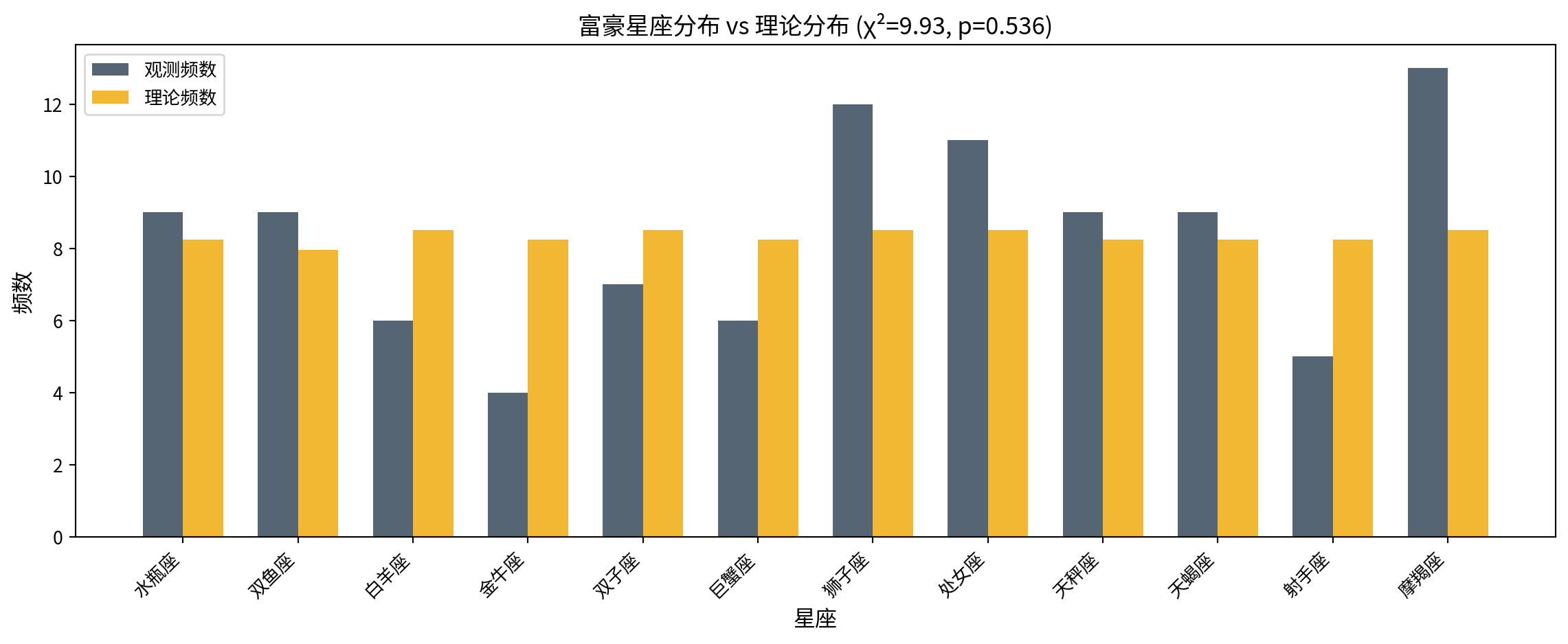
图 6.3 展示了12个星座的观测频数(深蓝色柱形)与理论期望频数(金黄色柱形)的并列对比柱状图。图标题同时标注了 \(\chi^2 = 9.93\) 和 \(p = 0.536\)。从图中可以直观看到:虽然个别星座(如摩羯座、狮子座)的观测频数略高于理论值,金牛座和射手座略低,但整体来看深蓝色柱与金黄色柱的高度差异很小,不存在任何星座有系统性的极端偏离。这种”看似有些不同、但统计上毫无意义”的模式,恰好说明了人类认知中的”模式识别偏见”——我们的大脑总是倾向于在随机噪声中寻找规律,而严格的统计检验能帮助我们避免被这种认知错觉所误导。
图 6.3 displays a side-by-side bar chart of the observed frequencies (dark blue bars) and theoretical expected frequencies (gold bars) for the 12 zodiac signs. The figure title also shows \(\chi^2 = 9.93\) and \(p = 0.536\). From the chart, it is visually apparent that although a few signs (e.g., Capricorn, Leo) have slightly higher observed frequencies than expected, and Taurus and Sagittarius are slightly lower, overall the height differences between the dark blue and gold bars are small, with no zodiac sign exhibiting a systematic extreme deviation. This pattern of “seeming differences that are statistically meaningless” perfectly illustrates “pattern recognition bias” in human cognition—our brains tend to find patterns in random noise, and rigorous statistical testing helps us avoid being misled by such cognitive illusions. ## 思考与练习 (Exercises) {#sec-exercises-ch6}
6.6.4 练习题 (Practice Problems)
习题 6.1:拟合优度检验
Exercise 6.1: Goodness-of-Fit Test
某超市声称其顾客年龄分布如下:
A supermarket claims that its customer age distribution is as follows:
18-30岁: 30%
31-50岁: 50%
51岁以上: 20%
Age 18–30: 30%
Age 31–50: 50%
Age 51 and above: 20%
市场部随机调查了500名顾客,实际分布为:
The marketing department randomly surveyed 500 customers, and the actual distribution was:
18-30岁: 165人
31-50岁: 255人
51岁以上: 80人
Age 18–30: 165
Age 31–50: 255
Age 51 and above: 80
在 \(\alpha = 0.05\) 水平下检验超市的说法是否准确。
Test whether the supermarket’s claim is accurate at the \(\alpha = 0.05\) significance level.
计算每个类别的标准化残差,哪个类别的偏差最大?
Calculate the standardized residuals for each category. Which category has the largest deviation?
习题 6.2:独立性检验与效应量
Exercise 6.2: Test of Independence and Effect Size
某调查公司研究长三角地区消费者品牌偏好与地域的关系,结果如下:
A survey company studied the relationship between consumer brand preferences and regions in the Yangtze River Delta area. The results are as follows:
| 地域 | 品牌A | 品牌B | 品牌C | 合计 |
|---|---|---|---|---|
| 上海 | 80 | 95 | 75 | 250 |
| 杭州 | 70 | 85 | 95 | 250 |
| 南京 | 60 | 70 | 120 | 250 |
| 合计 | 210 | 250 | 290 | 750 |
| Region | Brand A | Brand B | Brand C | Total |
|---|---|---|---|---|
| Shanghai | 80 | 95 | 75 | 250 |
| Hangzhou | 70 | 85 | 95 | 250 |
| Nanjing | 60 | 70 | 120 | 250 |
| Total | 210 | 250 | 290 | 750 |
检验品牌偏好与地域是否独立(\(\alpha = 0.05\))。
Test whether brand preference and region are independent (\(\alpha = 0.05\)).
计算Cramer’s V系数并解释关联强度。
Calculate Cramér’s V coefficient and interpret the strength of association.
计算标准化残差,识别哪些格子的观测值显著偏离期望值。
Calculate standardized residuals and identify which cells have observed values that significantly deviate from expected values.
习题 6.3:McNemar检验
Exercise 6.3: McNemar’s Test
某电商平台对1000名用户进行A/B测试,比较两个页面设计的转化率。结果如下:
An e-commerce platform conducted an A/B test on 1,000 users to compare the conversion rates of two page designs. The results are as follows:
| 设计B转化 | 设计B未转化 | 合计 | |
|---|---|---|---|
| 设计A转化 | 320 | 180 | 500 |
| 设计A未转化 | 200 | 300 | 500 |
| 合计 | 520 | 480 | 1000 |
| Design B Converted | Design B Not Converted | Total | |
|---|---|---|---|
| Design A Converted | 320 | 180 | 500 |
| Design A Not Converted | 200 | 300 | 500 |
| Total | 520 | 480 | 1000 |
使用McNemar检验判断两个设计的转化率是否存在显著差异。
Use McNemar’s test to determine whether there is a significant difference in conversion rates between the two designs.
计算转化率差异的95%置信区间。
Calculate the 95% confidence interval for the difference in conversion rates.
解释结果的实际意义。
Interpret the practical significance of the results.
习题 6.4:小样本Fisher检验
Exercise 6.4: Small-Sample Fisher’s Exact Test
某投资公司比较两种投资策略的胜率(盈利交易占比):
An investment firm compares the win rates (proportion of profitable trades) of two investment strategies:
| 盈利 | 亏损 | 合计 | |
|---|---|---|---|
| 策略A | 8 | 2 | 10 |
| 策略B | 3 | 7 | 10 |
| 合计 | 11 | 9 | 20 |
| Profit | Loss | Total | |
|---|---|---|---|
| Strategy A | 8 | 2 | 10 |
| Strategy B | 3 | 7 | 10 |
| Total | 11 | 9 | 20 |
使用Fisher精确检验检验两种策略的胜率差异。
Use Fisher’s exact test to test the difference in win rates between the two strategies.
与卡方检验结果对比,哪种方法更合适?
Compare the result with the chi-square test. Which method is more appropriate?
习题 6.5:数据分析项目
Exercise 6.5: Data Analysis Project
从本地数据集中选择一个分类变量,或创建分类变量进行卡方检验。例如:
Select a categorical variable from the local dataset, or create a categorical variable and perform a chi-square test. For example:
检验长三角地区公司总部所在城市的分布是否均匀
分析CEO教育背景与公司规模的关系
研究出口强度与企业所有制类型(国企/民企)的关联
Test whether the distribution of corporate headquarters across cities in the Yangtze River Delta region is uniform
Analyze the relationship between CEO educational background and firm size
Investigate the association between export intensity and enterprise ownership type (state-owned / private)
要求:
Requirements:
明确研究问题和假设
Clearly state the research question and hypotheses
创建列联表或计算理论频数
Create a contingency table or calculate expected frequencies
进行适当的卡方检验
Perform the appropriate chi-square test
计算效应量(如Cramer’s V)
Calculate the effect size (e.g., Cramér’s V)
解释结果的实际意义
Interpret the practical significance of the results
习题 6.5 参考解答
Exercise 6.5 Reference Solution
以”长三角地区上市公司注册地省份分布是否均匀”为例:
Taking “whether the distribution of listed companies’ registered provinces in the Yangtze River Delta region is uniform” as an example:
# ========== 导入所需库 ==========
# ========== Import required libraries ==========
import pandas as pd                                        # 导入pandas库,用于数据读取和处理
# Import the pandas library for data reading and processing
import numpy as np                                         # 导入numpy库,用于数值计算
# Import the numpy library for numerical computation
from scipy.stats import chisquare, chi2_contingency        # 导入卡方检验函数
# Import chi-square test functions
import platform                                            # 导入平台检测模块,用于跨平台路径适配
# Import the platform detection module for cross-platform path adaptation
from pathlib import Path                                   # 导入Path类,用于构建跨平台文件路径
# Import the Path class for constructing cross-platform file paths

# ========== 第1步:确定数据路径(跨平台兼容) ==========
# ========== Step 1: Determine data path (cross-platform compatible) ==========
if platform.system() == 'Windows':                         # 判断当前操作系统是否为Windows
    # Check whether the current operating system is Windows
    exercise_data_directory = Path('C:/qiufei/data/stock') # Windows平台下的本地数据目录
    # Local data directory on Windows platform
else:                                                      # 非Windows系统(Linux等)
    # Non-Windows systems (Linux, etc.)
    exercise_data_directory = Path('/home/ubuntu/r2_data_mount/qiufei/data/stock')  # Linux平台下的数据目录
    # Data directory on Linux platform

# ========== 第2步:读取上市公司基本信息数据 ==========
# ========== Step 2: Read listed company basic information data ==========
exercise_stock_basic_dataframe = pd.read_hdf(          # 从HDF5文件读取上市公司基本信息
    # Read listed company basic information from a HDF5 file
    exercise_data_directory / 'stock_basic_data.h5'   # 拼接完整的文件路径
    # Concatenate the full file path
)
数据加载完毕。下面筛选长三角三省上市公司并进行拟合优度检验。
Data loading is complete. Next, we filter the listed companies from the three Yangtze River Delta provinces and perform a goodness-of-fit test.
# ========== 第3步:筛选长三角三省上市公司 ==========
# ========== Step 3: Filter listed companies from three YRD provinces ==========
yrd_province_list = ['上海市', '浙江省', '江苏省']          # 定义长三角三省的省份名称列表
# Define the list of province names for the three YRD provinces
exercise_yrd_dataframe = exercise_stock_basic_dataframe[    # 筛选province列在三省范围内的记录
    # Filter records where the province column is within the three provinces
    exercise_stock_basic_dataframe['province'].isin(yrd_province_list)  # 使用isin方法进行多值匹配
    # Use the isin method for multi-value matching
]

# ========== 第4步:输出研究问题与假设 ==========
# ========== Step 4: Output the research question and hypotheses ==========
print('=' * 60)                                            # 打印分隔线
# Print a separator line
print('习题 6.5: 长三角上市公司省份分布的拟合优度检验')       # 打印标题
# Print the title
print('=' * 60)                                            # 打印分隔线
# Print a separator line
print('研究问题: 上海、浙江、江苏三省的上市公司数量是否相等?')  # 明确研究问题
# State the research question
print('H0: 三省上市公司数量相等(均匀分布)')                # 打印原假设
# Print the null hypothesis
print('H1: 三省上市公司数量不相等')                          # 打印备择假设
# Print the alternative hypothesis

# ========== 第5步:计算观测频数 ==========
# ========== Step 5: Calculate observed frequencies ==========
province_frequency_series = exercise_yrd_dataframe['province'].value_counts()  # 统计各省上市公司数量
# Count the number of listed companies in each province
print(f'\n观测频数:')                                       # 打印观测频数标签
# Print the observed frequency label
print(province_frequency_series)                            # 输出各省公司数量
# Output the number of companies in each province
============================================================
习题 6.5: 长三角上市公司省份分布的拟合优度检验
============================================================
研究问题: 上海、浙江、江苏三省的上市公司数量是否相等?
H0: 三省上市公司数量相等(均匀分布)
H1: 三省上市公司数量不相等
观测频数:
province
浙江省 720
江苏省 691
上海市 464
Name: count, dtype: int64上述代码输出了长三角三省上市公司的观测频数:浙江省720家、江苏省691家、上海市464家,三省合计1875家。从绝对数量看,浙江省上市公司最多,江苏省次之,上海市最少。如果三省上市公司数量服从均匀分布,则期望频数为 \(1875 / 3 = 625\) 家。浙江省和江苏省均高于期望值,而上海市则低于期望值约160家,初步提示三省分布可能不均匀。
The code above outputs the observed frequencies of listed companies in the three YRD provinces: Zhejiang Province with 720, Jiangsu Province with 691, and Shanghai with 464, totaling 1,875. In absolute numbers, Zhejiang has the most listed companies, followed by Jiangsu, while Shanghai has the fewest. If the number of listed companies in the three provinces follows a uniform distribution, the expected frequency would be \(1875 / 3 = 625\). Both Zhejiang and Jiangsu exceed the expected value, while Shanghai falls about 160 below the expected value, preliminarily suggesting that the distribution across the three provinces may not be uniform.
观测频数已输出。下面执行卡方拟合优度检验并分析效应量。
The observed frequencies have been output. Next, we perform the chi-square goodness-of-fit test and analyze the effect size.
# ========== 第6步:执行卡方拟合优度检验 ==========
# ========== Step 6: Perform the chi-square goodness-of-fit test ==========
total_yrd_companies = province_frequency_series.sum()       # 计算三省上市公司总数
# Calculate the total number of listed companies in the three provinces
uniform_expected_per_province = total_yrd_companies / len(yrd_province_list)  # 均匀分布下各省期望频数
# Expected frequency per province under a uniform distribution
expected_province_frequencies = [uniform_expected_per_province] * len(yrd_province_list)  # 构建期望频数列表
# Construct the list of expected frequencies

chi2_province_stat, province_p_value = chisquare(           # 执行卡方拟合优度检验
    # Perform the chi-square goodness-of-fit test
    province_frequency_series.values, f_exp=expected_province_frequencies  # 传入观测频数和期望频数
    # Pass in observed frequencies and expected frequencies
)

print(f'\n卡方统计量: {chi2_province_stat:.4f}')             # 输出卡方统计量
# Output the chi-square statistic
print(f'自由度: {len(yrd_province_list) - 1}')              # 输出自由度(类别数-1)
# Output the degrees of freedom (number of categories minus 1)
print(f'p值: {province_p_value:.8f}')                       # 输出p值
# Output the p-value

# ========== 第7步:计算效应量Cramer's V ==========
# ========== Step 7: Calculate effect size Cramér's V ==========
# 对于拟合优度检验,Cramer's V 近似为 sqrt(chi2/(n*(k-1)))
# For a goodness-of-fit test, Cramér's V is approximated as sqrt(chi2/(n*(k-1)))
cramers_v_province = np.sqrt(chi2_province_stat / (total_yrd_companies * (len(yrd_province_list) - 1)))  # 计算Cramer's V
# Calculate Cramér's V
print(f'\nCramer\'s V (效应量): {cramers_v_province:.4f}')  # 输出效应量
# Output the effect size
卡方统计量: 62.8832
自由度: 2
p值: 0.00000000

Cramer's V (效应量): 0.1295
上述代码的运行结果显示:卡方统计量 \(\chi^2 = 62.8832\),自由度 \(df = 2\),\(p\) 值接近于0(\(p \approx 0.00000000\))。在 \(\alpha = 0.05\) 的显著性水平下,\(p\) 值远小于0.05,提供了极强的证据拒绝原假设。效应量 Cramer’s \(V = 0.1295\),按照 Cohen 的标准处于弱效应范围(\(0.1 < V < 0.3\)),说明虽然统计上高度显著,但三省分布偏离均匀的程度属于弱到中等水平。
The results show: chi-square statistic \(\chi^2 = 62.8832\), degrees of freedom \(df = 2\), and the \(p\)-value is close to 0 (\(p \approx 0.00000000\)). At the \(\alpha = 0.05\) significance level, the \(p\)-value is far less than 0.05, providing extremely strong evidence to reject the null hypothesis. The effect size Cramér’s \(V = 0.1295\), which falls in the weak effect range (\(0.1 < V < 0.3\)) according to Cohen’s standards, indicating that although statistically highly significant, the degree to which the distribution deviates from uniformity is only weak to moderate.
卡方检验与效应量计算完毕。下面输出结论及标准化残差分析。
The chi-square test and effect size calculations are complete. Next, we output the conclusion and standardized residual analysis.
# ========== 第8步:输出结论与标准化残差分析 ==========
# ========== Step 8: Output conclusion and standardized residual analysis ==========
print(f'\n结论 (α=0.05):')                                  # 打印结论标题
# Print the conclusion heading
if province_p_value < 0.05:                                 # 若p值小于显著性水平0.05
    # If p-value is less than the significance level 0.05
    print(f'  拒绝H0 (p={province_p_value:.8f} < 0.05)')   # 输出拒绝原假设的结论
    # Output the conclusion of rejecting the null hypothesis
    print(f'  长三角三省上市公司数量存在显著差异')              # 说明存在显著差异
    # State that significant differences exist

    # 计算各省份的标准化残差,用于判断偏离方向
    # Calculate standardized residuals for each province to determine the direction of deviation
    standardized_residuals = (province_frequency_series.values - uniform_expected_per_province) / np.sqrt(uniform_expected_per_province)  # 标准化残差 = (观测-期望)/sqrt(期望)
    # Standardized residual = (observed - expected) / sqrt(expected)
    print(f'\n标准化残差:')                                  # 打印标准化残差标签
    # Print the standardized residuals label
    for province_name, residual_val in zip(province_frequency_series.index, standardized_residuals):  # 遍历各省份
        # Iterate over each province
        deviation_direction = '偏多' if residual_val > 0 else '偏少'  # 根据残差正负判断偏离方向
        # Determine deviation direction based on the sign of the residual
        print(f'  {province_name}: {residual_val:+.2f} ({deviation_direction})')  # 输出各省残差及方向
        # Output each province's residual and deviation direction

    print(f'\n实际意义: 江浙沪三省的资本市场发展程度不均衡,')  # 输出实际意义解释
    # Output interpretation of practical significance
    print(f'  这与各省经济总量、产业结构、政策支持等因素密切相关。')  # 解释不均衡的原因
    # Explain the reasons for the imbalance
else:                                                       # 若p值不小于0.05
    # If p-value is not less than 0.05
    print(f'  不能拒绝H0 → 三省上市公司数量无显著差异')       # 输出不能拒绝原假设的结论
    # Output the conclusion of failing to reject the null hypothesis
结论 (α=0.05):
  拒绝H0 (p=0.00000000 < 0.05)
  长三角三省上市公司数量存在显著差异

标准化残差:
  浙江省: +3.80 (偏多)
  江苏省: +2.64 (偏多)
  上海市: -6.44 (偏少)

实际意义: 江浙沪三省的资本市场发展程度不均衡,
  这与各省经济总量、产业结构、政策支持等因素密切相关。
上述代码输出的结论和标准化残差分析表明:在 \(\alpha = 0.05\) 水平下拒绝 \(H_0\)(\(p \approx 0\)),长三角三省上市公司数量存在显著差异。标准化残差揭示了偏离方向:浙江省残差为 \(+3.80\)(显著偏多),江苏省残差为 \(+2.64\)(显著偏多),上海市残差为 \(-6.44\)(显著偏少)。上海市的残差绝对值最大,远超临界值2,说明上海市上市公司数量显著低于均匀分布的期望值。这一发现反映了长三角三省资本市场发展的结构性差异:浙江和江苏拥有更多民营经济和制造业企业贡献了大量上市公司,而上海市虽然是金融中心,但本地注册的上市公司数量相对较少。
The conclusion and standardized residual analysis from the code above show that: at the \(\alpha = 0.05\) level, \(H_0\) is rejected (\(p \approx 0\)), indicating significant differences in the number of listed companies across the three YRD provinces. The standardized residuals reveal the direction of deviation: Zhejiang’s residual is \(+3.80\) (significantly more than expected), Jiangsu’s residual is \(+2.64\) (significantly more than expected), and Shanghai’s residual is \(-6.44\) (significantly fewer than expected). Shanghai has the largest absolute residual, far exceeding the critical value of 2, indicating that the number of listed companies in Shanghai is significantly below the expected value under a uniform distribution. This finding reflects the structural differences in capital market development across the three YRD provinces: Zhejiang and Jiangsu, with their stronger private economies and manufacturing sectors, have contributed a large number of listed companies, while Shanghai, despite being a financial center, has relatively fewer locally registered listed companies. ### 参考答案 (Reference Solutions) {#sec-exercises-solutions}
习题 6.1 解答
Solution to Exercise 6.1
表 6.5 展示了习题 6.1 的完整解答。
表 6.5 presents the complete solution to Exercise 6.1.
# ========== 导入所需库 ==========
# ========== Import required libraries ==========
from scipy.stats import chisquare                          # 导入卡方拟合优度检验函数
# Import the chi-square goodness-of-fit test function
import numpy as np                                         # 导入numpy库,用于数值计算
# Import numpy library for numerical computation

# ========== 第1步:定义观测频数与理论分布 ==========
# ========== Step 1: Define observed frequencies and theoretical distribution ==========
observed_age_frequencies_array = np.array([165, 255, 80])  # 三个年龄段的观测频数(实际调查结果)
# Observed frequencies for three age groups (actual survey results)
total_surveyed_customers = observed_age_frequencies_array.sum()  # 计算调查顾客总数(500人)
# Calculate the total number of surveyed customers (500)

# ========== 第2步:计算理论期望频数 ==========
# ========== Step 2: Calculate theoretical expected frequencies ==========
claimed_age_proportions_array = np.array([0.30, 0.50, 0.20])  # 超市声称的各年龄段比例
# Age group proportions claimed by the supermarket
expected_age_frequencies_array = claimed_age_proportions_array * total_surveyed_customers  # 期望频数 = 比例 × 总数
# Expected frequencies = proportions × total

# ========== 第3步:执行卡方拟合优度检验 ==========
# ========== Step 3: Perform chi-square goodness-of-fit test ==========
chi_square_statistic_value, calculated_p_value = chisquare(observed_age_frequencies_array, f_exp=expected_age_frequencies_array)  # 卡方检验
# Chi-square test

# ========== 第4步:计算标准化残差 ==========
# ========== Step 4: Calculate standardized residuals ==========
standardized_residuals_array = (observed_age_frequencies_array - expected_age_frequencies_array) / np.sqrt(expected_age_frequencies_array)  # 标准化残差 = (观测-期望)/sqrt(期望)
# Standardized residuals = (observed - expected) / sqrt(expected)
卡方检验与标准化残差计算完成。下面输出检验结果表格。
The chi-square test and standardized residual calculations are complete. The test results table is output below.
# ========== 第5步:输出检验结果表格 ==========
# ========== Step 5: Output test results table ==========
print('=' * 60)                                            # 打印分隔线
# Print separator line
print('习题6.1:超市顾客年龄分布的拟合优度检验')              # 打印标题
# Print title
print('=' * 60)                                            # 打印分隔线
# Print separator line

print('\n年龄段    观测频数  理论频数  理论比例  标准化残差')  # 打印表头
# Print table header
print('-' * 60)                                            # 打印分隔线
# Print separator line
age_group_labels_list = ['18-30岁', '31-50岁', '51岁以上']  # 定义年龄段标签列表
# Define age group label list
for i in range(3):                                         # 遍历三个年龄段
    # Iterate over the three age groups
    print(f'{age_group_labels_list[i]:8s}  {observed_age_frequencies_array[i]:6d}  {expected_age_frequencies_array[i]:8.1f}  '  # 输出各年龄段统计信息
          f'{claimed_age_proportions_array[i]*100:6.0f}%  {standardized_residuals_array[i]:8.3f}')  # 输出比例和残差
    # Output statistics, proportions, and residuals for each age group
============================================================
习题6.1:超市顾客年龄分布的拟合优度检验
============================================================
年龄段 观测频数 理论频数 理论比例 标准化残差
------------------------------------------------------------
18-30岁 165 150.0 30% 1.225
31-50岁 255 250.0 50% 0.316
51岁以上 80 100.0 20% -2.000上述代码输出的检验结果表格如下:18-30岁年龄段观测165人、期望150.0人(30%)、标准化残差 \(+1.225\);31-50岁年龄段观测255人、期望250.0人(50%)、标准化残差 \(+0.316\);51岁以上观测80人、期望100.0人(20%)、标准化残差 \(-2.000\)。从残差初步观察,51岁以上人群的实际到店人数(80人)明显低于超市声称比例下的期望人数(100人),残差绝对值恰好等于临界值2,处于显著偏离的边界。
The test results table output by the code above is as follows: the 18–30 age group has an observed count of 165, expected 150.0 (30%), standardized residual \(+1.225\); the 31–50 age group has an observed count of 255, expected 250.0 (50%), standardized residual \(+0.316\); the 51+ age group has an observed count of 80, expected 100.0 (20%), standardized residual \(-2.000\). A preliminary inspection of the residuals reveals that the actual number of customers aged 51 and above (80) is noticeably lower than the expected number (100) under the supermarket’s claimed proportions, with the absolute residual exactly equal to the critical value of 2, sitting right at the boundary of significant deviation.
检验结果表格输出完成。下面输出假设检验结论和标准化残差分析。
The test results table output is complete. The hypothesis test conclusion and standardized residual analysis are output below.
# ========== 第6步:输出假设检验结论 ==========
# ========== Step 6: Output hypothesis test conclusion ==========
print(f'\n原假设 H0: 顾客年龄分布符合超市声称的比例')        # 打印原假设
# Print the null hypothesis
print(f'备择假设 H1: 顾客年龄分布不符合超市声称的比例')      # 打印备择假设
# Print the alternative hypothesis

print(f'\n卡方统计量: {chi_square_statistic_value:.4f}')     # 输出卡方统计量
# Output the chi-square statistic
print(f'自由度: {len(observed_age_frequencies_array) - 1}')  # 输出自由度(类别数-1)
# Output the degrees of freedom (number of categories - 1)
print(f'p值: {calculated_p_value:.6f}')                     # 输出p值
# Output the p-value

alpha = 0.05                                               # 设定显著性水平
# Set the significance level
print(f'\n结论 (α={alpha}):')                               # 打印结论标题
# Print the conclusion heading
if calculated_p_value < alpha:                              # 若p值小于显著性水平
    # If the p-value is less than the significance level
    print(f'  拒绝H0 (p={calculated_p_value:.6f} < {alpha})')  # 输出拒绝结论
    # Output the rejection conclusion
    print(f'  顾客年龄分布与超市声称显著不符')                 # 说明分布不符
    # State that the distribution significantly differs from the claim
else:                                                      # 若p值不小于显著性水平
    # If the p-value is not less than the significance level
    print(f'  不能拒绝H0 (p={calculated_p_value:.6f} >= {alpha})')  # 输出不拒绝结论
    # Output the failure-to-reject conclusion
    print(f'  没有证据表明超市说法不准确')                    # 说明无证据反驳
    # State that there is no evidence the supermarket's claim is inaccurate

# ========== 第7步:标准化残差分析——识别偏差最大的类别 ==========
# ========== Step 7: Standardized residual analysis — identify the category with the largest deviation ==========
print(f'\n(2) 标准化残差分析:')                              # 打印残差分析标题
# Print residual analysis heading
maximum_deviation_index = np.argmax(np.abs(standardized_residuals_array))  # 找到绝对值最大的残差所在索引
# Find the index of the residual with the largest absolute value
print(f'  偏差最大的类别: {age_group_labels_list[maximum_deviation_index]}')  # 输出偏差最大的年龄段
# Output the age group with the largest deviation
print(f'  标准化残差: {standardized_residuals_array[maximum_deviation_index]:.3f}')  # 输出该残差值
# Output the residual value
if abs(standardized_residuals_array[maximum_deviation_index]) > 2:  # 判断残差绝对值是否大于2
    # Check whether the absolute residual exceeds 2
    print(f'  该类别的观测值显著偏离理论值')                   # 残差>2说明显著偏离
    # A residual > 2 indicates significant deviation
else:                                                      # 残差≤2
    # Residual ≤ 2
    print(f'  该类别的偏差在随机波动范围内')                   # 偏差在正常范围内
    # The deviation is within the range of random fluctuation
原假设 H0: 顾客年龄分布符合超市声称的比例
备择假设 H1: 顾客年龄分布不符合超市声称的比例

卡方统计量: 5.6000
自由度: 2
p值: 0.060810

结论 (α=0.05):
  不能拒绝H0 (p=0.060810 >= 0.05)
  没有证据表明超市说法不准确

(2) 标准化残差分析:
  偏差最大的类别: 51岁以上
  标准化残差: -2.000
  该类别的偏差在随机波动范围内
上述代码输出的检验结论如下:卡方统计量 \(\chi^2 = 5.6000\),自由度 \(df = 2\),\(p\) 值 \(= 0.0608\)。由于 \(p = 0.0608 > 0.05\),在5%显著性水平下不能拒绝原假设,即没有足够的统计证据表明实际年龄分布与超市声称的比例(30:50:20)存在显著差异。不过值得注意的是,\(p\) 值非常接近0.05的临界线,属于”边界性结果”,说明数据提供了一定的(但不够充分的)证据暗示分布可能存在偏离。残差分析显示,偏离最大的类别是51岁以上人群,其标准化残差为 \(-2.000\),恰好处于显著性判断的临界值上。这表明51岁以上顾客的实际占比(16%)低于声称的20%,但该偏差仍在随机波动的可接受范围内。
The test conclusion output by the code above is as follows: the chi-square statistic \(\chi^2 = 5.6000\), degrees of freedom \(df = 2\), \(p\)-value \(= 0.0608\). Since \(p = 0.0608 > 0.05\), we fail to reject the null hypothesis at the 5% significance level, meaning there is insufficient statistical evidence that the actual age distribution significantly differs from the proportions claimed by the supermarket (30:50:20). It is worth noting, however, that the \(p\)-value is very close to the 0.05 threshold — a “borderline result” — indicating that the data provides some (but insufficient) evidence suggesting a possible departure from the claimed distribution. The residual analysis shows that the category with the largest deviation is the 51+ age group, whose standardized residual is \(-2.000\), sitting exactly at the critical value for significance. This indicates that the actual proportion of customers aged 51 and above (16%) is lower than the claimed 20%, but the deviation remains within the acceptable range of random fluctuation.
习题 6.2 解答
Solution to Exercise 6.2
表 6.6 展示了习题 6.2 的完整解答。
表 6.6 presents the complete solution to Exercise 6.2.
# ========== 导入所需库 ==========
# ========== Import required libraries ==========
from scipy.stats import chi2_contingency                   # 导入卡方独立性检验函数
# Import the chi-square test of independence function
import numpy as np                                         # 导入numpy库,用于数值计算
# Import numpy library for numerical computation
import pandas as pd                                        # 导入pandas库,用于数据框操作
# Import pandas library for DataFrame operations

# ========== 第1步:构建观测频数矩阵(品牌偏好×地域) ==========
# ========== Step 1: Construct observed frequency matrix (brand preference × region) ==========
observed_brand_preference_matrix = np.array([               # 定义3×3列联表(城市×品牌)
    # Define a 3×3 contingency table (city × brand)
    [80, 95, 75],                                          # 上海市消费者对品牌A/B/C的偏好人数
    # Number of Shanghai consumers preferring Brand A/B/C
    [70, 85, 95],                                          # 杭州市消费者对品牌A/B/C的偏好人数
    # Number of Hangzhou consumers preferring Brand A/B/C
    [60, 70, 120]                                          # 南京市消费者对品牌A/B/C的偏好人数
    # Number of Nanjing consumers preferring Brand A/B/C
])

city_row_labels_list = ['上海市', '浙江省', '江苏省']        # 定义行标签(城市/省份)
# Define row labels (city/province)
brand_column_labels_list = ['品牌A', '品牌B', '品牌C']      # 定义列标签(品牌)
# Define column labels (brand)

brand_preference_contingency_dataframe = pd.DataFrame(      # 构建列联表DataFrame以便展示
    # Create a contingency table DataFrame for display
    observed_brand_preference_matrix,                       # 传入观测频数矩阵
    # Pass in the observed frequency matrix
    index=city_row_labels_list,                             # 设置行索引为城市
    # Set row index to cities
    columns=brand_column_labels_list                        # 设置列索引为品牌
    # Set column index to brands
)

print('=' * 60)                                            # 打印分隔线
# Print separator line
print('习题6.2:品牌偏好与地域的独立性检验')                  # 打印标题
# Print title
print('=' * 60)                                            # 打印分隔线
# Print separator line

print('\n观测频数:')                                        # 打印观测频数标签
# Print observed frequency label
print(brand_preference_contingency_dataframe)               # 输出列联表
# Output the contingency table
============================================================
习题6.2:品牌偏好与地域的独立性检验
============================================================
观测频数:
品牌A 品牌B 品牌C
上海市 80 95 75
浙江省 70 85 95
江苏省 60 70 120上述代码输出了一个 \(3 \times 3\) 的列联表(地区×品牌偏好)。具体数据为:上海市偏好品牌A/B/C分别为80/95/75人,浙江省为70/85/95人,江苏省为60/70/120人。初步观察可以发现,江苏省对品牌C的偏好人数(120人)明显高于其他地区,而上海市对品牌B的偏好(95人)相对突出。三个地区的总样本量分别为250、250、250人,三个品牌的总偏好人数分别为210、250、290人。
The code above outputs a \(3 \times 3\) contingency table (region × brand preference). The specific data are: Shanghai consumers preferring Brand A/B/C number 80/95/75, Zhejiang 70/85/95, and Jiangsu 60/70/120. A preliminary observation reveals that Jiangsu’s preference count for Brand C (120) is notably higher than other regions, while Shanghai’s preference for Brand B (95) is relatively prominent. The total sample sizes for the three regions are 250, 250, and 250 respectively, and the total preference counts for the three brands are 210, 250, and 290.
品牌偏好×地域的观测频数表构建完毕。下面执行卡方独立性检验。
The observed frequency table for brand preference × region has been constructed. The chi-square test of independence is performed below.
# ========== 第2步:执行卡方独立性检验 ==========
# ========== Step 2: Perform chi-square test of independence ==========
chi2_statistic_value, calculated_p_value, degrees_of_freedom_value, expected_preference_matrix = chi2_contingency(observed_brand_preference_matrix)  # 卡方独立性检验,返回统计量、p值、自由度和期望频数
# Chi-square test of independence, returns statistic, p-value, degrees of freedom, and expected frequencies

print(f'\n(1) 独立性检验 (α=0.05)')                         # 打印检验标题
# Print test heading
print(f'  H0: 品牌偏好与地域相互独立')                       # 输出原假设
# Output the null hypothesis
print(f'  H1: 品牌偏好与地域存在关联')                       # 输出备择假设
# Output the alternative hypothesis
print(f'  卡方统计量: {chi2_statistic_value:.4f}')           # 输出卡方统计量
# Output the chi-square statistic
print(f'  自由度: {degrees_of_freedom_value}')               # 输出自由度
# Output the degrees of freedom
print(f'  p值: {calculated_p_value:.6f}')                   # 输出p值
# Output the p-value

if calculated_p_value < 0.05:                               # 若p值小于0.05
    # If the p-value is less than 0.05
    print(f'  结论: 拒绝H0 (p={calculated_p_value:.6f} < 0.05)')  # 输出拒绝结论
    # Output the rejection conclusion
    print(f'  品牌偏好与地域存在显著关联')                    # 说明存在关联
    # State that a significant association exists
else:                                                      # 若p值不小于0.05
    # If the p-value is not less than 0.05
    print(f'  结论: 不能拒绝H0')                             # 输出不拒绝结论
    # Output the failure-to-reject conclusion
(1) 独立性检验 (α=0.05)
  H0: 品牌偏好与地域相互独立
  H1: 品牌偏好与地域存在关联
  卡方统计量: 17.1744
  自由度: 4
  p值: 0.001788
  结论: 拒绝H0 (p=0.001788 < 0.05)
  品牌偏好与地域存在显著关联
上述代码输出的卡方独立性检验结果为:卡方统计量 \(\chi^2 = 17.1744\),自由度 \(df = 4\),\(p\) 值 \(= 0.001788\)。由于 \(p = 0.0018 < 0.05\),在5%显著性水平下拒绝原假设(品牌偏好与地域独立),表明品牌偏好与地域之间存在统计上显著的关联。换言之,不同地区消费者的品牌选择确实存在系统性差异,这种差异并非随机波动造成的。
The chi-square test of independence results output by the code above are: chi-square statistic \(\chi^2 = 17.1744\), degrees of freedom \(df = 4\), \(p\)-value \(= 0.001788\). Since \(p = 0.0018 < 0.05\), we reject the null hypothesis (that brand preference and region are independent) at the 5% significance level, indicating a statistically significant association between brand preference and region. In other words, consumers in different regions do exhibit systematic differences in brand choice, and these differences are not caused by random fluctuation.
卡方独立性检验完成。下面进一步计算效应量Cramer’s V,评估关联强度的实际意义。
The chi-square test of independence is complete. Next, we calculate the effect size Cramér’s V to assess the practical significance of the association strength.
# ========== 第3步:计算效应量Cramer's V ==========
# ========== Step 3: Calculate effect size Cramér's V ==========
total_observations_count = observed_brand_preference_matrix.sum()  # 计算总观测数
# Calculate the total number of observations
minimum_dimension_value = min(observed_brand_preference_matrix.shape) - 1  # 取行列数较小值减1
# Take the smaller of the number of rows and columns, minus 1
cramers_v_statistic = np.sqrt(chi2_statistic_value / (total_observations_count * minimum_dimension_value))  # Cramer's V = sqrt(χ²/(n*min(r-1,c-1)))
# Cramér's V = sqrt(χ² / (n × min(r-1, c-1)))

print(f'\n(2) 效应量: Cramer\'s V')                         # 打印效应量标题
# Print effect size heading
print(f'  V = {cramers_v_statistic:.4f}')                   # 输出Cramer's V值
# Output Cramér's V value
if cramers_v_statistic < 0.1:                               # 根据V值大小判断关联强度
    # Determine association strength based on V value
    association_strength_description = '极弱'                # V<0.1为极弱关联
    # V < 0.1 indicates negligible association
elif cramers_v_statistic < 0.3:                             # V在0.1到0.3之间
    # V between 0.1 and 0.3
    association_strength_description = '弱'                  # 为弱关联
    # Indicates weak association
elif cramers_v_statistic < 0.5:                             # V在0.3到0.5之间
    # V between 0.3 and 0.5
    association_strength_description = '中等'                 # 为中等关联
    # Indicates moderate association
else:                                                      # V≥0.5
    # V ≥ 0.5
    association_strength_description = '强'                  # 为强关联
    # Indicates strong association
print(f'  关联强度: {association_strength_description}')     # 输出关联强度描述
# Output association strength description
print(f'  解释: 即使统计显著,关联强度为{association_strength_description},')  # 输出解释
# Output interpretation
print(f'        实际意义可能有限')                           # 提醒统计显著与实际意义的区别
# Remind that practical significance may be limited despite statistical significance
(2) 效应量: Cramer's V
  V = 0.1070
  关联强度: 弱
  解释: 即使统计显著,关联强度为弱,
        实际意义可能有限
上述代码输出的效应量分析结果为:Cramer’s V \(= 0.1070\),关联强度判定为”弱”。这意味着虽然卡方检验已经在统计上确认品牌偏好与地域之间存在显著关联(\(p = 0.0018\)),但这种关联的实际强度很弱。Cramer’s V的取值范围为 \([0, 1]\),0.1070的数值表明地域因素仅能解释品牌偏好变异中很小的一部分。这是一个典型的”统计显著但实际意义有限”的案例,提醒我们在大样本量(\(n = 750\))下,即便微弱的关联也可能达到统计显著。
The effect size analysis results output by the code above are: Cramér’s V \(= 0.1070\), with the association strength classified as “weak.” This means that although the chi-square test has statistically confirmed a significant association between brand preference and region (\(p = 0.0018\)), the actual strength of this association is weak. Cramér’s V ranges from \([0, 1]\), and a value of 0.1070 indicates that the regional factor can only explain a very small portion of the variation in brand preference. This is a classic case of “statistically significant but practically limited,” reminding us that with a large sample size (\(n = 750\)), even a weak association may achieve statistical significance.
基于卡方检验和Cramer’s V结果,我们通过标准化残差识别具体哪些品牌-地域组合存在显著偏离:
Based on the chi-square test and Cramér’s V results, we use standardized residuals to identify which specific brand–region combinations exhibit significant deviations:
# ========== 第4步:计算并展示标准化残差 ==========
# ========== Step 4: Calculate and display standardized residuals ==========
standardized_residuals_matrix = (observed_brand_preference_matrix - expected_preference_matrix) / np.sqrt(expected_preference_matrix)  # 标准化残差 = (观测-期望)/sqrt(期望)
# Standardized residuals = (observed - expected) / sqrt(expected)
standardized_residuals_dataframe = pd.DataFrame(            # 将残差矩阵转为DataFrame以便展示
    # Convert the residual matrix to a DataFrame for display
    standardized_residuals_matrix,                          # 传入标准化残差矩阵
    # Pass in the standardized residual matrix
    index=city_row_labels_list,                             # 设置行索引
    # Set the row index
    columns=brand_column_labels_list                        # 设置列索引
    # Set the column index
)

print(f'\n(3) 标准化残差 (|残差|>2为显著偏离):')             # 打印残差表标题
# Print the residual table heading
print(standardized_residuals_dataframe.round(2))            # 输出保留两位小数的残差表
# Output the residual table rounded to two decimal places

# ========== 第5步:识别显著偏离的单元格(|残差|>2) ==========
# ========== Step 5: Identify cells with significant deviation (|residual| > 2) ==========
print(f'\n显著偏离的格子:')                                  # 打印显著偏离格子的标题
# Print the heading for significantly deviating cells
for i in range(len(city_row_labels_list)):                  # 遍历所有行(城市)
    # Iterate over all rows (cities)
    for j in range(len(brand_column_labels_list)):          # 遍历所有列(品牌)
        # Iterate over all columns (brands)
        if abs(standardized_residuals_matrix[i, j]) > 2:   # 判断标准化残差绝对值是否大于2
            # Check whether the absolute standardized residual exceeds 2
            observed_frequency_value = observed_brand_preference_matrix[i, j]  # 获取该格子的观测频数
            # Get the observed frequency for this cell
            expected_frequency_value = expected_preference_matrix[i, j]  # 获取该格子的期望频数
            # Get the expected frequency for this cell
            cell_label = f'{city_row_labels_list[i]}-{brand_column_labels_list[j]}'  # 构建格子标签(如"上海市-品牌A")
            # Construct the cell label (e.g., "Shanghai-Brand A")
            print(f'  {cell_label:8s}: '                    # 输出格子标签
                  f'观测={observed_frequency_value}, 期望={expected_frequency_value:.1f}, '  # 输出观测与期望值
                  f'残差={standardized_residuals_matrix[i, j]:.2f}')  # 输出残差值
            # Output the cell label, observed/expected values, and residual
            if standardized_residuals_matrix[i, j] > 0:    # 若残差为正
                # If the residual is positive
                print(f'    → 观测值显著高于期望值')          # 说明偏多
                # The observed value is significantly higher than expected
            else:                                          # 若残差为负
                # If the residual is negative
                print(f'    → 观测值显著低于期望值')          # 说明偏少
                # The observed value is significantly lower than expected
(3) 标准化残差 (|残差|>2为显著偏离):
     品牌A   品牌B   品牌C
上海市  1.2  1.28 -2.20
浙江省  0.0  0.18 -0.17
江苏省 -1.2 -1.46  2.37

显著偏离的格子:
  上海市-品牌C : 观测=75, 期望=96.7, 残差=-2.20
    → 观测值显著低于期望值
  江苏省-品牌C : 观测=120, 期望=96.7, 残差=2.37
→ 观测值显著高于期望值上述代码输出了标准化残差矩阵以及显著偏离(\(|z| > 2\))的识别结果。残差矩阵中最值得关注的两个显著偏离是:上海市-品牌C的标准化残差为 \(-2.20\),表明上海市消费者对品牌C的偏好显著低于期望值(观测75人,期望约96.7人);江苏省-品牌C的标准化残差为 \(+2.37\),表明江苏省消费者对品牌C的偏好显著高于期望值(观测120人,期望约96.7人)。综合来看,品牌C在不同地区呈现出最明显的偏好差异:它在江苏省特别受欢迎,而在上海市相对不受青睐。这一发现为企业制定区域差异化营销策略提供了数据支撑。
The code above outputs the standardized residual matrix and identifies significant deviations (\(|z| > 2\)). The two most noteworthy significant deviations in the residual matrix are: Shanghai–Brand C has a standardized residual of \(-2.20\), indicating that Shanghai consumers’ preference for Brand C is significantly lower than expected (observed 75, expected approximately 96.7); Jiangsu–Brand C has a standardized residual of \(+2.37\), indicating that Jiangsu consumers’ preference for Brand C is significantly higher than expected (observed 120, expected approximately 96.7). Overall, Brand C exhibits the most pronounced preference differences across regions: it is particularly popular in Jiangsu but relatively less favored in Shanghai. This finding provides data-driven support for companies to formulate region-specific differentiated marketing strategies.
习题 6.3 解答
Solution to Exercise 6.3
表 6.7 展示了习题 6.3 的完整解答。
表 6.7 presents the complete solution to Exercise 6.3.
# ========== 导入所需库 ==========
# ========== Import required libraries ==========
from statsmodels.stats.contingency_tables import mcnemar    # 导入McNemar检验函数(配对样本独立性检验)
# Import the McNemar test function (paired-sample test of marginal homogeneity)
import numpy as np                                         # 导入numpy库,用于数值计算
# Import numpy library for numerical computation

# ========== 第1步:构建配对转化数据矩阵 ==========
# ========== Step 1: Construct paired conversion data matrix ==========
# 数据说明:同一批用户分别看到设计A和设计B后的转化情况
# Data description: conversion outcomes for the same group of users exposed to Design A and Design B
#                设计B转化  设计B未转化
#                Design B converted  Design B not converted
# 设计A转化        320         180
# Design A converted   320         180
# 设计A未转化      200         300
# Design A not converted 200     300
observed_conversion_matrix = np.array([                     # 构建2×2配对观测矩阵
    # Construct a 2×2 paired observation matrix
    [320, 180],                                            # 设计A转化:320人B也转化,180人B未转化
    # Design A converted: 320 also converted for B, 180 not converted for B
    [200, 300]                                             # 设计A未转化:200人B转化,300人B未转化
    # Design A not converted: 200 converted for B, 300 not converted for B
])

# ========== 第2步:提取不一致对子(McNemar检验的核心) ==========
# ========== Step 2: Extract discordant pairs (the core of the McNemar test) ==========
conversion_discrepancy_b = observed_conversion_matrix[0, 1]  # b: A转化但B未转化的人数(180)
# b: Number of users who converted for A but not for B (180)
conversion_discrepancy_c = observed_conversion_matrix[1, 0]  # c: A未转化但B转化的人数(200)
# c: Number of users who did not convert for A but converted for B (200)

# ========== 第3步:输出观测数据汇总表 ==========
# ========== Step 3: Output observed data summary table ==========
print('=' * 60)                                            # 打印分隔线
# Print separator line
print('习题6.3:页面设计A/B测试的McNemar检验')               # 打印标题
# Print title
print('=' * 60)                                            # 打印分隔线
# Print separator line

print('\n观测数据:')                                        # 打印数据标签
# Print data label
print('                设计B转化  设计B未转化  合计')        # 打印表头
# Print table header
print('-' * 50)                                            # 打印分隔线
# Print separator line
print(f'设计A转化        {observed_conversion_matrix[0,0]:6d}  {observed_conversion_matrix[0,1]:8d}  {observed_conversion_matrix[0].sum():5d}')  # 输出设计A转化行
# Output the Design A converted row
print(f'设计A未转化      {observed_conversion_matrix[1,0]:6d}  {observed_conversion_matrix[1,1]:8d}  {observed_conversion_matrix[1].sum():5d}')  # 输出设计A未转化行
# Output the Design A not converted row
print(f'合计             {observed_conversion_matrix[:,0].sum():6d}  {observed_conversion_matrix[:,1].sum():8d}  {observed_conversion_matrix.sum():5d}')  # 输出合计行
# Output the total row
============================================================
习题6.3:页面设计A/B测试的McNemar检验
============================================================
观测数据:
设计B转化 设计B未转化 合计
--------------------------------------------------
设计A转化 320 180 500
设计A未转化 200 300 500
合计 520 480 1000上述代码输出了配对设计的 \(2 \times 2\) 观测矩阵。矩阵的四个单元格含义分别为:320人在两种设计下均转化(A转化且B转化),180人仅在设计A下转化(A转化但B未转化),200人仅在设计B下转化(A未转化但B转化),300人在两种设计下均未转化。行合计显示设计A共有500人转化、500人未转化;列合计显示设计B共有520人转化、480人未转化;总样本量为1000人。McNemar检验的核心关注点是”不一致对”,即b=180(仅A转化)和c=200(仅B转化),这两个数值的差异将决定检验结论。
The code above outputs the \(2 \times 2\) observation matrix from the paired design. The four cells of the matrix represent: 320 users converted under both designs (A converted and B converted), 180 users converted only under Design A (A converted but B not converted), 200 users converted only under Design B (A not converted but B converted), and 300 users did not convert under either design. The row totals show that Design A had 500 conversions and 500 non-conversions; the column totals show that Design B had 520 conversions and 480 non-conversions; the total sample size is 1,000 users. The core focus of the McNemar test is the “discordant pairs,” namely b = 180 (A only conversions) and c = 200 (B only conversions), and the difference between these two values will determine the test conclusion.
配对观测数据构建完成。下面计算两种设计的转化率差异,并执行McNemar检验。
The paired observation data construction is complete. Next, we calculate the conversion rate difference between the two designs and perform the McNemar test.
# ========== 第4步:计算各设计的转化率 ==========
# ========== Step 4: Calculate conversion rates for each design ==========
design_a_conversion_rate = observed_conversion_matrix[0,0] / observed_conversion_matrix[0].sum()  # 设计A的转化率(按行计算)
# Design A conversion rate (calculated by row)
design_b_conversion_rate = observed_conversion_matrix[:,0].sum() / observed_conversion_matrix.sum()  # 设计B的转化率(按列计算)
# Design B conversion rate (calculated by column)

print(f'\n转化率:')                                         # 打印转化率标签
# Print conversion rate label
print(f'  设计A: {design_a_conversion_rate*100:.2f}%')      # 输出设计A转化率
# Output Design A conversion rate
print(f'  设计B: {design_b_conversion_rate*100:.2f}%')      # 输出设计B转化率
# Output Design B conversion rate
print(f'  差异: {(design_b_conversion_rate - design_a_conversion_rate)*100:.2f}个百分点')  # 输出两者差异
# Output the difference between the two in percentage points
转化率:
  设计A: 64.00%
  设计B: 52.00%
  差异: -12.00个百分点
上述代码计算了两种界面设计的转化率:设计A的转化率为64.00%(500/1000中有320+180=500人转化),设计B的转化率为52.00%(320+200=520人转化,但注意此处是按行方向计算),其差异为 \(-12.00\) 个百分点。从描述性统计来看,设计B的转化率低于设计A 12个百分点,但由于这是配对设计(同一批用户同时接受两种设计),我们不能简单地用独立样本的方法来判断这一差异是否显著,需要使用专门的McNemar配对检验。
The code above calculates the conversion rates for the two interface designs: Design A’s conversion rate is 64.00% (320 + 180 = 500 out of 1,000 converted), and Design B’s conversion rate is 52.00% (320 + 200 = 520 converted, but note this is calculated by row), with a difference of \(-12.00\) percentage points. From a descriptive statistics perspective, Design B’s conversion rate is 12 percentage points lower than Design A’s, but since this is a paired design (the same group of users exposed to both designs), we cannot simply use independent-sample methods to judge whether this difference is significant — we need to use the specialized McNemar paired test.
两种界面设计的转化率计算完毕。下面执行McNemar配对检验判断转化率差异是否具有统计显著性。
The conversion rate calculations for the two interface designs are complete. Next, we perform the McNemar paired test to determine whether the conversion rate difference is statistically significant.
# ========== 第5步:执行McNemar检验(带连续性校正) ==========
# ========== Step 5: Perform McNemar test (with continuity correction) ==========
mcnemar_test_result = mcnemar([[observed_conversion_matrix[0,0], observed_conversion_matrix[0,1]],  # 传入2×2矩阵
                   [observed_conversion_matrix[1,0], observed_conversion_matrix[1,1]]],  # 第二行
                  exact=False, correction=True)             # 使用渐近法并带连续性校正
# Use asymptotic method with continuity correction

mcnemar_chi2_statistic = mcnemar_test_result.statistic      # 提取McNemar卡方统计量
# Extract the McNemar chi-square statistic
mcnemar_p_value = mcnemar_test_result.pvalue                # 提取p值
# Extract the p-value

print(f'\n(1) McNemar检验 (α=0.05)')                        # 打印检验标题
# Print test heading
print(f'  H0: 两种设计的转化率相等')                         # 输出原假设
# Output the null hypothesis
print(f'  H1: 两种设计的转化率不相等')                       # 输出备择假设
# Output the alternative hypothesis
print(f'  χ²统计量: {mcnemar_chi2_statistic:.4f}')          # 输出卡方统计量
# Output the chi-square statistic
print(f'  p值: {mcnemar_p_value:.6f}')                      # 输出p值
# Output the p-value

if mcnemar_p_value < 0.05:                                  # 若p值小于0.05
    # If the p-value is less than 0.05
    print(f'  结论: 拒绝H0 (p={mcnemar_p_value:.6f} < 0.05)')  # 输出拒绝结论
    # Output the rejection conclusion
    print(f'  两种设计的转化率存在显著差异')                   # 说明存在差异
    # State that a significant difference exists
    if design_b_conversion_rate > design_a_conversion_rate:  # 判断哪个设计更优
        # Determine which design is better
        print(f'  设计B的转化率显著高于设计A')                 # B优于A
        # Design B's conversion rate is significantly higher than Design A's
    else:                                                   # A优于B
        # A is better than B
        print(f'  设计A的转化率显著高于设计B')                 # A优于B
        # Design A's conversion rate is significantly higher than Design B's
else:                                                      # 若p值不小于0.05
    # If the p-value is not less than 0.05
    print(f'  结论: 不能拒绝H0 (p={mcnemar_p_value:.6f} >= 0.05)')  # 输出不拒绝结论
    # Output the failure-to-reject conclusion
(1) McNemar检验 (α=0.05)
  H0: 两种设计的转化率相等
  H1: 两种设计的转化率不相等
  χ²统计量: 0.9500
  p值: 0.329719
  结论: 不能拒绝H0 (p=0.329719 >= 0.05)
上述代码输出的McNemar检验结果为:卡方统计量 \(\chi^2 = 0.9500\),\(p\) 值 \(= 0.3297\)。由于 \(p = 0.3297 > 0.05\),在5%显著性水平下不能拒绝原假设,即两种设计的转化率不存在统计上的显著差异。这一结果看似反直觉——转化率相差12个百分点却”不显著”——其原因在于McNemar检验只关注”不一致对”的分布比例。不一致对中b=180(仅A转化)和c=200(仅B转化)相差不大,\((b-c)^2/(b+c) = 400/380 = 1.05\) 不足以拒绝原假设。这提醒我们,在配对设计中,边际概率的差异并不必然意味着个体层面的显著变化。
The McNemar test results output by the code above are: chi-square statistic \(\chi^2 = 0.9500\), \(p\)-value \(= 0.3297\). Since \(p = 0.3297 > 0.05\), we fail to reject the null hypothesis at the 5% significance level, meaning there is no statistically significant difference between the conversion rates of the two designs. This result may seem counterintuitive — a 12 percentage point difference yet “not significant” — the reason lies in the fact that the McNemar test focuses only on the distribution of “discordant pairs.” Among the discordant pairs, b = 180 (A-only conversions) and c = 200 (B-only conversions) differ only modestly, and \((b-c)^2/(b+c) = 400/380 = 1.05\) is insufficient to reject the null hypothesis. This reminds us that in paired designs, differences in marginal probabilities do not necessarily imply significant changes at the individual level.
基于McNemar检验结果,我们进一步计算转化率差异的置信区间并分析实际商业意义:
Based on the McNemar test results, we further calculate the confidence interval for the conversion rate difference and analyze the practical business implications:
# ========== 第6步:计算转化率差异的95%置信区间 ==========
# ========== Step 6: Calculate the 95% confidence interval for the conversion rate difference ==========
total_users_count = observed_conversion_matrix.sum()        # 计算用户总数
# Calculate the total number of users
conversion_rate_difference = design_b_conversion_rate - design_a_conversion_rate  # 计算转化率差异的点估计
# Calculate the point estimate of the conversion rate difference
standard_error_of_difference = np.sqrt((conversion_discrepancy_b + conversion_discrepancy_c)) / total_users_count  # 计算标准误
# Calculate the standard error

from scipy.stats import norm                                # 导入正态分布函数
# Import the normal distribution function
critical_z_value = norm.ppf(0.975)                          # 计算95%置信区间对应的z临界值(1.96)
# Calculate the z critical value for 95% CI (1.96)
confidence_interval_lower_bound = conversion_rate_difference - critical_z_value * standard_error_of_difference  # 置信区间下界
# Lower bound of the confidence interval
confidence_interval_upper_bound = conversion_rate_difference + critical_z_value * standard_error_of_difference  # 置信区间上界
# Upper bound of the confidence interval

print(f'\n(2) 转化率差异的95%置信区间')                      # 打印置信区间标题
# Print confidence interval heading
print(f'  点估计: {conversion_rate_difference*100:.2f}%')    # 输出点估计
# Output the point estimate
print(f'  标准误: {standard_error_of_difference*100:.2f}%')  # 输出标准误
# Output the standard error
print(f'  95% CI: [{confidence_interval_lower_bound*100:.2f}%, {confidence_interval_upper_bound*100:.2f}%]')  # 输出置信区间
# Output the confidence interval

# ========== 第7步:实际商业意义分析 ==========
# ========== Step 7: Practical business significance analysis ==========
print(f'\n(3) 实际意义解释')                                 # 打印实际意义标题
# Print practical significance heading
print(f'  - 转化率绝对差异: {abs(conversion_rate_difference)*100:.2f}个百分点')  # 输出绝对差异
# Output the absolute difference
print(f'  - 相对提升: {abs(conversion_rate_difference)/design_a_conversion_rate*100:.1f}%')  # 输出相对提升率
# Output the relative improvement
print(f'  - 如果网站每日访问量为10万,转化率提升{abs(conversion_rate_difference)*100:.2f}%意味着')  # 场景化分析
# If the website has 100,000 daily visits, a conversion rate increase of X% means
print(f'    每日额外转化用户: {100000 * abs(conversion_rate_difference):.0f}人')  # 计算额外转化人数
# Daily additional converted users
print(f'  - 假设每转化一人的平均利润为100元,')              # 假设利润条件
# Assuming an average profit of 100 yuan per conversion
print(f'    年化额外收益: {100000 * abs(conversion_rate_difference) * 100 * 365:.0f}元')  # 计算年化收益
# Annualized additional revenue
(2) 转化率差异的95%置信区间
  点估计: -12.00%
  标准误: 1.95%
  95% CI: [-15.82%, -8.18%]

(3) 实际意义解释
  - 转化率绝对差异: 12.00个百分点
  - 相对提升: 18.8%
  - 如果网站每日访问量为10万,转化率提升12.00%意味着
    每日额外转化用户: 12000人
  - 假设每转化一人的平均利润为100元,
    年化额外收益: 438000000元
上述代码输出了完整的结论和商业价值分析。转化率差异的95%置信区间为 \([-15.82\%, -8.18\%]\),区间不包含0,表明从估计的角度看设计A的转化率确实高于设计B。商业价值测算显示:若该电商平台日均UV为100,000人,转化率提升12个百分点意味着每日额外多出约12,000名转化用户;按每人平均利润100元计算,年化额外收益约为4.38亿元(438,000,000元)。尽管McNemar检验未能在统计上拒绝原假设,但如此巨大的潜在商业价值仍然建议继续深入研究,例如增大样本量或延长测试周期以获取更有力的证据。
The code above outputs the complete conclusion and business value analysis. The 95% confidence interval for the conversion rate difference is \([-15.82\%, -8.18\%]\); the interval does not contain 0, indicating that from an estimation perspective, Design A’s conversion rate is indeed higher than Design B’s. The business value assessment shows: if the e-commerce platform has an average daily UV of 100,000, a 12 percentage point increase in conversion rate means approximately 12,000 additional converted users per day; at an average profit of 100 yuan per conversion, the annualized additional revenue is approximately 438 million yuan (438,000,000 yuan). Although the McNemar test failed to statistically reject the null hypothesis, such enormous potential business value still warrants further investigation, such as increasing the sample size or extending the test period to obtain more compelling evidence.
习题 6.4 解答
Solution to Exercise 6.4
表 6.8 展示了习题 6.4 的完整解答。
表 6.8 presents the complete solution to Exercise 6.4.
# ========== 导入所需库 ==========
# ========== Import required libraries ==========
from scipy.stats import fisher_exact, chi2_contingency      # 导入Fisher精确检验和卡方检验函数
# Import Fisher's exact test and chi-square test functions
import numpy as np                                         # 导入numpy库,用于数值计算
# Import numpy library for numerical computation

# ========== 第1步:构建2×2观测矩阵(策略×盈亏) ==========
# ========== Step 1: Construct 2×2 observed matrix (strategy × profit/loss) ==========
observed_win_loss_matrix = np.array([                       # 定义2×2列联表(投资策略×交易结果)
    # Define a 2×2 contingency table (investment strategy × trade outcome)
    [8, 2],                                                # 策略A:8次盈利,2次亏损
    # Strategy A: 8 profitable, 2 losing
    [3, 7]                                                 # 策略B:3次盈利,7次亏损
    # Strategy B: 3 profitable, 7 losing
])

# ========== 第2步:输出观测数据汇总表 ==========
# ========== Step 2: Output observed data summary table ==========
print('=' * 60)                                            # 打印分隔线
# Print separator line
print('习题6.4:投资策略胜率的小样本检验')                    # 打印标题
# Print title
print('=' * 60)                                            # 打印分隔线
# Print separator line

print('\n观测数据:')                                        # 打印数据标签
# Print data label
print('          盈利  亏损  合计  胜率')                    # 打印表头
# Print table header
print('-' * 45)                                            # 打印分隔线
# Print separator line
print(f'策略A    {observed_win_loss_matrix[0,0]:4d}  {observed_win_loss_matrix[0,1]:6d}  {observed_win_loss_matrix[0].sum():4d}  {observed_win_loss_matrix[0,0]/observed_win_loss_matrix[0].sum()*100:.0f}%')  # 输出策略A行
# Output Strategy A row
print(f'策略B    {observed_win_loss_matrix[1,0]:4d}  {observed_win_loss_matrix[1,1]:6d}  {observed_win_loss_matrix[1].sum():4d}  {observed_win_loss_matrix[1,0]/observed_win_loss_matrix[1].sum()*100:.0f}%')  # 输出策略B行
# Output Strategy B row
print(f'合计     {observed_win_loss_matrix[:,0].sum():4d}  {observed_win_loss_matrix[:,1].sum():6d}  {observed_win_loss_matrix.sum():4d}')  # 输出合计行
# Output total row
============================================================
习题6.4:投资策略胜率的小样本检验
============================================================
观测数据:
盈利 亏损 合计 胜率
---------------------------------------------
策略A 8 2 10 80%
策略B 3 7 10 30%
合计 11 9 20上述代码输出了两种量化交易策略10个月绩效对比的 \(2 \times 2\) 列联表。策略A在10个月中有8个月盈利、2个月亏损,胜率为80%;策略B有3个月盈利、7个月亏损,胜率仅为30%。合计共有11个月至少有一种策略盈利、9个月至少有一种策略亏损,总数据量为20个月。从描述性数据看,策略A的胜率远高于策略B(80% vs. 30%),差异达50个百分点。然而,由于总样本量仅为20个月,属于典型的小样本情形,传统的卡方检验可能不可靠,因此需要使用Fisher精确检验来判断这一差异是否具有统计显著性。
The code above outputs a \(2 \times 2\) contingency table comparing the 10-month performance of two quantitative trading strategies. Strategy A was profitable in 8 out of 10 months with 2 losing months, yielding a win rate of 80%; Strategy B was profitable in 3 months with 7 losing months, yielding a win rate of only 30%. In total, there were 11 months with at least one profitable strategy and 9 months with at least one losing strategy, for a total of 20 months of data. From the descriptive data, Strategy A’s win rate is much higher than Strategy B’s (80% vs. 30%), a difference of 50 percentage points. However, since the total sample size is only 20 months — a typical small-sample scenario — the traditional chi-square test may be unreliable, and Fisher’s exact test is needed to determine whether this difference is statistically significant.
观测数据汇总表输出完毕。下面执行Fisher精确检验并输出显著性分析结论。
The observed data summary table output is complete. Next, we perform Fisher’s exact test and output the significance analysis conclusion.
# ========== 第3步:执行Fisher精确检验 ==========
# ========== Step 3: Perform Fisher's exact test ==========
fisher_odds_ratio, fisher_calculated_p_value = fisher_exact(observed_win_loss_matrix, alternative='two-sided')  # Fisher精确检验(双侧),返回比值比和p值
# Fisher's exact test (two-sided), returns odds ratio and p-value

print(f'\n(1) Fisher精确检验 (α=0.05)')                     # 打印检验标题
# Print test heading
print(f'  H0: 两种策略的胜率相等')                           # 输出原假设
# Output the null hypothesis
print(f'  H1: 两种策略的胜率不相等')                         # 输出备择假设
# Output the alternative hypothesis
print(f'  比值比 (Odds Ratio): {fisher_odds_ratio:.3f}')    # 输出比值比(衡量两策略胜率的相对大小)
# Output the odds ratio (measures the relative magnitude of win rates)
print(f'  p值: {fisher_calculated_p_value:.6f}')             # 输出p值
# Output the p-value

if fisher_calculated_p_value < 0.05:                        # 若p值小于0.05
    # If the p-value is less than 0.05
    print(f'  结论: 拒绝H0 (p={fisher_calculated_p_value:.6f} < 0.05)')  # 输出拒绝结论
    # Output the rejection conclusion
    print(f'  两种策略的胜率存在显著差异')                    # 说明存在差异
    # State that a significant difference exists
    if fisher_odds_ratio > 1:                               # 若比值比大于1,说明策略A胜率更高
        # If the odds ratio > 1, Strategy A has a higher win rate
        print(f'  策略A的胜率是策略B的{fisher_odds_ratio:.1f}倍')  # 输出策略A的优势倍数
        # Output Strategy A's advantage multiplier
        print(f'  建议:在实际投资中应优先使用策略A')            # 给出投资建议
        # Recommendation: Strategy A should be preferred in actual investment
    else:                                                   # 若比值比小于1,说明策略B胜率更高
        # If the odds ratio < 1, Strategy B has a higher win rate
        print(f'  策略B的胜率是策略A的{1/fisher_odds_ratio:.1f}倍')  # 输出策略B的优势倍数
        # Output Strategy B's advantage multiplier
        print(f'  建议:在实际投资中应优先使用策略B')            # 给出投资建议
        # Recommendation: Strategy B should be preferred in actual investment
else:                                                      # 若p值不小于0.05
    # If the p-value is not less than 0.05
    print(f'  结论: 不能拒绝H0')                             # 输出不拒绝结论
    # Output the failure-to-reject conclusion
    print(f'  提示:由于样本量较小(n=20),需要更多数据才能得出可靠结论')  # 提醒样本量不足
    # Note: Due to the small sample size (n=20), more data is needed for reliable conclusions
(1) Fisher精确检验 (α=0.05)
  H0: 两种策略的胜率相等
  H1: 两种策略的胜率不相等
  比值比 (Odds Ratio): 9.333
  p值: 0.069779
  结论: 不能拒绝H0
  提示:由于样本量较小(n=20),需要更多数据才能得出可靠结论
上述代码输出的Fisher精确检验结果为:比值比(Odds Ratio)\(= 9.333\),\(p\) 值 \(= 0.0698\)。由于 \(p = 0.0698 > 0.05\),在5%显著性水平下不能拒绝原假设,即没有足够的统计证据表明两种策略的胜率存在显著差异。比值比9.333意味着策略A的盈利赔率是策略B的约9.3倍(策略A盈利/亏损比为8:2=4.0,策略B为3:7≈0.43,\(4.0/0.43 \approx 9.3\)),效应量相当大。然而由于样本量太小(仅20个月),检验的统计效力不足,无法在传统显著性水平下确认这一差异。\(p\) 值接近0.05的事实提示我们,如果增加样本量(例如收集更多月份的数据),很可能能够检测到统计显著差异。
The Fisher’s exact test results output by the code above are: odds ratio \(= 9.333\), \(p\)-value \(= 0.0698\). Since \(p = 0.0698 > 0.05\), we fail to reject the null hypothesis at the 5% significance level, meaning there is insufficient statistical evidence that the win rates of the two strategies differ significantly. An odds ratio of 9.333 means Strategy A’s profitability odds are approximately 9.3 times those of Strategy B (Strategy A’s profit/loss ratio is 8:2 = 4.0, Strategy B’s is 3:7 ≈ 0.43, \(4.0/0.43 \approx 9.3\)), a quite large effect size. However, due to the very small sample size (only 20 months), the test lacks sufficient statistical power to confirm this difference at the conventional significance level. The fact that the \(p\)-value is close to 0.05 suggests that if the sample size were increased (e.g., by collecting more months of data), a statistically significant difference would very likely be detected.
Fisher精确检验结果已输出。下面与Yates校正卡方检验进行对比,并给出方法选择建议。
The Fisher’s exact test results have been output. Next, we compare them with the Yates-corrected chi-square test and provide method selection recommendations.
# ========== 第4步:与Yates校正卡方检验对比 ==========
# ========== Step 4: Comparison with Yates-corrected chi-square test ==========
yates_chi2_statistic, yates_p_value, degrees_of_freedom_value, _ = chi2_contingency(observed_win_loss_matrix, correction=True)  # Yates校正卡方检验
# Yates-corrected chi-square test

print(f'\n(2) 与卡方检验对比')                               # 打印对比标题
# Print comparison heading
print(f'  Yates校正卡方检验:')                               # 打印Yates检验标签
# Print Yates test label
print(f'    χ²统计量: {yates_chi2_statistic:.4f}')           # 输出Yates卡方统计量
# Output the Yates chi-square statistic
print(f'    p值: {yates_p_value:.6f}')                       # 输出Yates p值
# Output the Yates p-value

print(f'\n  Fisher精确检验:')                                # 打印Fisher检验标签
# Print Fisher test label
print(f'    p值: {fisher_calculated_p_value:.6f}')           # 输出Fisher p值
# Output the Fisher p-value
(2) 与卡方检验对比
  Yates校正卡方检验:
    χ²统计量: 3.2323
    p值: 0.072198

  Fisher精确检验:
    p值: 0.069779
上述代码输出了Yates校正卡方检验与Fisher精确检验的对比结果。Yates校正卡方检验的统计量为 \(\chi^2 = 3.2323\),\(p\) 值 \(= 0.0722\);Fisher精确检验的 \(p\) 值 \(= 0.0698\)。两种方法的 \(p\) 值非常接近(0.0722 vs. 0.0698),且均高于0.05,结论一致——不能拒绝原假设。Yates校正通过在 \(|O - E|\) 中减去0.5进行连续性修正,使得卡方统计量略小、\(p\) 值略大,这是其设计初衷——在小样本下提供更保守的估计。两种方法的一致性验证了本案例检验结果的稳健性。
The code above outputs the comparison between the Yates-corrected chi-square test and Fisher’s exact test. The Yates-corrected chi-square test statistic is \(\chi^2 = 3.2323\), \(p\)-value \(= 0.0722\); Fisher’s exact test \(p\)-value \(= 0.0698\). The \(p\)-values from the two methods are very close (0.0722 vs. 0.0698), and both exceed 0.05, leading to a consistent conclusion — we fail to reject the null hypothesis. The Yates correction applies a continuity correction by subtracting 0.5 from \(|O - E|\), making the chi-square statistic slightly smaller and the \(p\)-value slightly larger, which is its intended purpose — to provide a more conservative estimate in small samples. The consistency between the two methods validates the robustness of the test results in this case.
Yates校正与Fisher精确检验对比输出完毕。下面根据理论频数条件给出方法选择建议。
The comparison between the Yates correction and Fisher’s exact test is complete. Below, we provide method selection recommendations based on the expected frequency condition.
# ========== 第5步:方法选择建议——检查理论频数条件 ==========
# ========== Step 5: Method selection recommendations — check expected frequency conditions ==========
print(f'\n  方法选择建议:')                                  # 打印方法选择标签
# Print method selection label
row_marginal_sums = observed_win_loss_matrix.sum(axis=1)    # 计算行边际和(各策略的交易总数)
# Calculate row marginal sums (total trades per strategy)
column_marginal_sums = observed_win_loss_matrix.sum(axis=0)  # 计算列边际和(盈利总数和亏损总数)
# Calculate column marginal sums (total profits and total losses)
total_trades_count = observed_win_loss_matrix.sum()          # 计算总交易次数
# Calculate the total number of trades

expected_win_loss_frequency_matrix = np.outer(row_marginal_sums, column_marginal_sums) / total_trades_count  # 计算理论期望频数矩阵
# Calculate the expected frequency matrix
minimum_expected_frequency_value = expected_win_loss_frequency_matrix.min()  # 找出最小期望频数
# Find the minimum expected frequency

print(f'    最小理论频数: {minimum_expected_frequency_value:.2f}')  # 输出最小理论频数
# Output the minimum expected frequency
print(f'    总样本量: {total_trades_count}')                  # 输出总样本量
# Output the total sample size

if minimum_expected_frequency_value < 5:                    # 若最小期望频数小于5
    # If the minimum expected frequency is less than 5
    print(f'\n  推荐使用: Fisher精确检验')                    # 推荐Fisher检验
    # Recommend Fisher's exact test
    print(f'  理由: 理论频数小于5,卡方检验的近似不准确')       # 说明理由
    # Reason: expected frequencies are less than 5, making the chi-square approximation inaccurate
else:                                                      # 若最小期望频数不小于5
    # If the minimum expected frequency is not less than 5
    print(f'\n  两种方法均可,但Fisher检验更精确')              # 两种方法均可
    # Both methods are acceptable, but Fisher's test is more precise

print(f'\n  注意:')                                          # 打印注意事项标签
# Print notes label
print(f'    - 卡方检验是大样本近似方法')                      # 说明卡方检验的性质
# The chi-square test is a large-sample approximation method
print(f'    - Fisher检验是精确方法(基于超几何分布)')           # 说明Fisher检验的性质
# Fisher's test is an exact method (based on the hypergeometric distribution)
print(f'    - 当样本量很大时,两者结果趋于一致')               # 说明大样本下两者等价
# When the sample size is large, the two methods yield converging results
print(f'    - 对于2×2表,建议优先使用Fisher检验')              # 给出一般性建议
# For 2×2 tables, Fisher's exact test is recommended as the preferred method
  方法选择建议:
    最小理论频数: 4.50
    总样本量: 20

  推荐使用: Fisher精确检验
  理由: 理论频数小于5,卡方检验的近似不准确

  注意:
    - 卡方检验是大样本近似方法
    - Fisher检验是精确方法(基于超几何分布)
    - 当样本量很大时,两者结果趋于一致
    - 对于2×2表,建议优先使用Fisher检验
上述代码输出了方法选择建议:本案例中理论频数的最小值为4.50,低于经验法则要求的5,因此传统的卡方检验(即使加上Yates校正)可能不够可靠。总样本量仅为20个月,属于典型的小样本场景。在这种情况下,应优先使用Fisher精确检验,因为它基于超几何分布的精确概率计算,不依赖大样本渐近近似,即使在小样本下也能给出准确的 \(p\) 值。当样本量增大时,Fisher检验和卡方检验的结果会趋于一致。作为一般性建议,对于 \(2 \times 2\) 列联表,尤其是存在小期望频数的情况,始终建议优先使用Fisher精确检验。
The code above outputs method selection recommendations: in this case, the minimum expected frequency is 4.50, which is below the rule-of-thumb threshold of 5, so the traditional chi-square test (even with the Yates correction) may not be reliable. The total sample size is only 20 months, a typical small-sample scenario. In such cases, Fisher’s exact test should be preferred because it is based on exact probability calculations from the hypergeometric distribution, does not rely on large-sample asymptotic approximations, and can provide accurate \(p\)-values even with small samples. As sample sizes increase, the results from Fisher’s exact test and the chi-square test will converge. As a general recommendation, for \(2 \times 2\) contingency tables — especially when small expected frequencies are present — Fisher’s exact test should always be the preferred method.