# ========== 导入所需库 ==========
# ========== Import required libraries ==========
import pandas as pd                    # 数据处理与分析
                                       # Data processing and analysis
import numpy as np                     # 数值计算
                                       # Numerical computation
import statsmodels.api as sm           # 统计建模(OLS回归等)
                                       # Statistical modeling (OLS regression, etc.)
from scipy import stats                # 科学计算(统计检验等)
                                       # Scientific computing (statistical tests, etc.)
import matplotlib.pyplot as plt        # 数据可视化
                                       # Data visualization
import platform                        # 系统平台检测
                                       # System platform detection

# ========== 中文字体设置 ==========
# ========== Chinese font configuration ==========
if platform.system() == 'Linux':       # Linux系统字体配置
                                       # Linux system font configuration
    plt.rcParams['font.sans-serif'] = ['Source Han Serif SC', 'SimHei', 'DejaVu Sans']  # 设置Linux下中文字体优先级
                                                                                         # Set Chinese font priority on Linux
else:                                  # Windows系统字体配置
                                       # Windows system font configuration
    plt.rcParams['font.sans-serif'] = ['SimHei', 'Microsoft YaHei']  # 设置Windows下中文字体优先级
                                                                      # Set Chinese font priority on Windows
plt.rcParams['axes.unicode_minus'] = False  # 解决负号显示问题
                                             # Fix minus sign display issue

# ========== 数据路径设置 ==========
# ========== Data path configuration ==========
if platform.system() == 'Linux':       # Linux平台数据路径
                                       # Linux platform data path
    data_path = '/home/ubuntu/r2_data_mount/qiufei/data/stock'  # Linux平台的股票数据存储路径
                                                                  # Stock data storage path on Linux
else:                                  # Windows平台数据路径
                                       # Windows platform data path
    data_path = 'C:/qiufei/data/stock'  # Windows平台的股票数据存储路径
                                         # Stock data storage path on Windows

# ========== 第1步:读取财务数据与公司基本信息 ==========
# ========== Step 1: Read financial data and company basic information ==========
financial_statement_dataframe = pd.read_hdf(f'{data_path}/financial_statement.h5')  # 读取上市公司财务报表
                                                                                             # Read listed company financial statements
stock_basic_info_dataframe = pd.read_hdf(f'{data_path}/stock_basic_data.h5')        # 读取股票基本信息
# Read stock basic information10 多元线性回归模型 (Multiple Linear Regression Models)
多元线性回归(Multiple Linear Regression)是研究一个因变量与多个自变量之间线性关系的统计方法。它是计量经济学、金融分析和商业预测的核心工具,允许我们在控制其他变量的情况下,估计每个自变量对因变量的净效应(Net Effect)。
Multiple Linear Regression is a statistical method for studying the linear relationship between one dependent variable and multiple independent variables. It is a core tool in econometrics, financial analysis, and business forecasting, allowing us to estimate the net effect of each independent variable on the dependent variable while controlling for other variables.
10.1 多元回归在公司金融研究中的典型应用 (Typical Applications of Multiple Regression in Corporate Finance Research)
多元线性回归是公司金融实证研究和多因子资产定价的核心工具。以下展示其在中国上市公司分析中的典型应用。
Multiple linear regression is a core tool for empirical corporate finance research and multi-factor asset pricing. The following demonstrates its typical applications in the analysis of Chinese listed companies.
10.1.1 应用一:Fama-French多因子模型 (Application 1: Fama-French Multi-Factor Model)
单因子CAPM模型(参见 章节 8 )往往无法完全解释股票收益率的截面差异。Fama-French三因子模型通过加入规模因子(SMB)和价值因子(HML),将单因子回归扩展为多元回归:
The single-factor CAPM model (see 章节 8) often cannot fully explain the cross-sectional variation in stock returns. The Fama-French three-factor model extends the single-factor regression into a multiple regression by adding a size factor (SMB) and a value factor (HML):
\[ R_{i,t} - R_{f,t} = \alpha_i + \beta_{i,m}(R_{m,t} - R_{f,t}) + \beta_{i,s} SMB_t + \beta_{i,h} HML_t + \varepsilon_{i,t} \]
利用 valuation_factors_quarterly_15_years.h5 中的估值因子数据和 stock_price_pre_adjusted.h5 中的行情数据,可以为A股市场构建多因子模型,检验各因子的显著性和解释力。
Using the valuation factor data in valuation_factors_quarterly_15_years.h5 and the market data in stock_price_pre_adjusted.h5, one can construct a multi-factor model for the A-share market to test the significance and explanatory power of each factor.
10.1.2 应用二:上市公司盈利能力的多因素分析 (Application 2: Multi-Factor Analysis of Listed Company Profitability)
什么因素决定了上市公司的盈利能力?利用 financial_statement.h5 中的面板数据,以ROE为因变量,以公司规模(总资产对数)、资产周转率、资产负债率、研发投入比等为自变量进行多元回归。通过分析每个因素的回归系数及其统计显著性,可以识别出对盈利能力影响最大的关键因素,为企业经营決策提供实证依据。这一分析的关键优势在于多元回归能够控制其他变量,估计每个因素的净效应。
What factors determine the profitability of listed companies? Using the panel data in financial_statement.h5, one can perform a multiple regression with ROE as the dependent variable and company size (log of total assets), asset turnover, debt-to-asset ratio, R&D intensity, etc. as independent variables. By analyzing the regression coefficient and statistical significance of each factor, the key factors with the greatest impact on profitability can be identified, providing empirical evidence for corporate decision-making. The key advantage of this analysis is that multiple regression can control for other variables and estimate the net effect of each factor.
10.1.3 从简单回归到多元回归 (From Simple Regression to Multiple Regression)
简单线性回归只考虑一个自变量:
Simple linear regression considers only one independent variable:
\[ Y = \beta_0 + \beta_1 X + \varepsilon \]
但现实中,因变量通常受多个因素影响。例如,公司盈利能力(ROE)可能同时受到公司规模、资产周转率、财务杠杆等多因素影响。多元回归让我们能够:
However, in reality, the dependent variable is usually influenced by multiple factors. For example, company profitability (ROE) may be simultaneously affected by company size, asset turnover, financial leverage, and other factors. Multiple regression enables us to:
控制混杂变量: 分离出每个变量的净效应
提高解释力: 捕获更多影响因素
进行因果推断: 在观测数据中近似实验效果
Control for confounding variables: Isolate the net effect of each variable
Improve explanatory power: Capture more influencing factors
Conduct causal inference: Approximate experimental effects in observational data
什么是混杂变量(Confounder)?
What Is a Confounder?
混杂变量是指同时影响自变量和因变量的第三方变量。如果不控制混杂变量,就会导致对自变量和因变量之间真实关系的错误估计——这种错误被称为遗漏变量偏误(Omitted Variable Bias, OVB)。
A confounder is a third-party variable that simultaneously affects both the independent and dependent variables. Failing to control for confounders leads to erroneous estimation of the true relationship between the independent and dependent variables — this error is called Omitted Variable Bias (OVB).
举一个中国上市公司研究中的典型例子:假设我们想研究”研发投入”对”公司利润”的影响。如果模型中只有这两个变量,可能会发现正相关关系。但仔细想想,“公司规模”同时影响了研发投入(大公司研发投入多)和利润(大公司利润高)。此处”公司规模”就是一个混杂变量。如果不在回归模型中控制它,研发投入的系数就包含了部分”规模效应”,从而高估了研发投入的真实影响。多元回归通过将混杂变量纳入模型,“剥离”其对因变量的影响,从而得到自变量的净效应(偏回归系数)。
Consider a typical example from Chinese listed company research: suppose we want to study the effect of “R&D investment” on “company profit.” If only these two variables are in the model, a positive correlation might be found. But think carefully — “company size” simultaneously affects both R&D investment (larger firms invest more in R&D) and profit (larger firms have higher profits). Here, “company size” is a confounder. If it is not controlled for in the regression model, the coefficient of R&D investment will include part of the “size effect,” thereby overestimating the true impact of R&D investment. By incorporating confounders into the model, multiple regression “strips away” their effect on the dependent variable, yielding the net effect (partial regression coefficient) of the independent variable.
10.2 模型设定 (Model Specification)
10.2.1 标准形式 (Standard Form)
多元线性回归模型的标量形式(式 10.1):
The scalar form of the multiple linear regression model (式 10.1):
\[ Y_i = \beta_0 + \beta_1 X_{i1} + \beta_2 X_{i2} + ... + \beta_p X_{ip} + \varepsilon_i, \quad i=1,2,...,n \tag{10.1}\]
10.2.2 矩阵形式 (Matrix Form)
为了方便推导和计算,我们使用矩阵形式(式 10.2):
For convenience in derivation and computation, we use the matrix form (式 10.2):
\[ \mathbf{Y} = \mathbf{X}\boldsymbol{\beta} + \boldsymbol{\varepsilon} \tag{10.2}\]
其中:
where:
\[ \mathbf{Y} = \begin{pmatrix} Y_1 \\ Y_2 \\ \vdots \\ Y_n \end{pmatrix}_{n \times 1}, \quad \mathbf{X} = \begin{pmatrix} 1 & X_{11} & X_{12} & \cdots & X_{1p} \\ 1 & X_{21} & X_{22} & \cdots & X_{2p} \\ \vdots & \vdots & \vdots & \ddots & \vdots \\ 1 & X_{n1} & X_{n2} & \cdots & X_{np} \end{pmatrix}_{n \times (p+1)} \]
\[ \boldsymbol{\beta} = \begin{pmatrix} \beta_0 \\ \beta_1 \\ \vdots \\ \beta_p \end{pmatrix}_{(p+1) \times 1}, \quad \boldsymbol{\varepsilon} = \begin{pmatrix} \varepsilon_1 \\ \varepsilon_2 \\ \vdots \\ \varepsilon_n \end{pmatrix}_{n \times 1} \]
10.2.3 经典假设 (Classical Assumptions)
经典线性回归模型(CLRM)基于以下假设:
The Classical Linear Regression Model (CLRM) is based on the following assumptions:
线性性: \(E(Y|X) = \mathbf{X}\boldsymbol{\beta}\) (条件期望是自变量的线性函数)
严格外生性: \(E(\varepsilon_i | \mathbf{X}) = 0\) (误差项与自变量不相关)
无完全多重共线性: \(\text{rank}(\mathbf{X}) = p+1\) (设计矩阵满秩)
同方差性: \(\text{Var}(\varepsilon_i | \mathbf{X}) = \sigma^2\) (误差方差恒定)
无自相关: \(\text{Cov}(\varepsilon_i, \varepsilon_j | \mathbf{X}) = 0, \forall i \neq j\)
正态性: \(\varepsilon | \mathbf{X} \sim N(0, \sigma^2 \mathbf{I}_n)\) (误差服从正态分布)
Linearity: \(E(Y|X) = \mathbf{X}\boldsymbol{\beta}\) (The conditional expectation is a linear function of the independent variables)
Strict exogeneity: \(E(\varepsilon_i | \mathbf{X}) = 0\) (The error term is uncorrelated with the independent variables)
No perfect multicollinearity: \(\text{rank}(\mathbf{X}) = p+1\) (The design matrix has full rank)
Homoscedasticity: \(\text{Var}(\varepsilon_i | \mathbf{X}) = \sigma^2\) (The error variance is constant)
No autocorrelation: \(\text{Cov}(\varepsilon_i, \varepsilon_j | \mathbf{X}) = 0, \forall i \neq j\)
Normality: \(\varepsilon | \mathbf{X} \sim N(0, \sigma^2 \mathbf{I}_n)\) (The errors follow a normal distribution)
假设的重要性与后果
Importance and Consequences of the Assumptions
| 假设 | 违反后果 | 检验方法 |
|---|---|---|
| 线性性 | 估计有偏 | 残差图、RESET检验 |
| 外生性 | 估计有偏且不一致 | 工具变量法 |
| 满秩 | 无法估计 | VIF检验 |
| 同方差性 | 标准误有偏 | BP检验、White检验 |
| 无自相关 | 标准误有偏 | DW检验、LM检验 |
| 正态性 | 小样本推断失效 | Shapiro-Wilk检验 |
| Assumption | Consequence of Violation | Test Method |
|---|---|---|
| Linearity | Biased estimates | Residual plots, RESET test |
| Exogeneity | Biased and inconsistent estimates | Instrumental variables |
| Full rank | Cannot estimate | VIF test |
| Homoscedasticity | Biased standard errors | BP test, White test |
| No autocorrelation | Biased standard errors | DW test, LM test |
| Normality | Small-sample inference fails | Shapiro-Wilk test |
理解这些假设对于正确应用回归分析至关重要。后续章节将详细讨论假设违反时的诊断和补救方法。
Understanding these assumptions is crucial for the correct application of regression analysis. Subsequent sections will discuss in detail the diagnostic and remedial methods when assumptions are violated.
10.3 最小二乘估计 (Ordinary Least Squares Estimation)
10.3.1 OLS估计量的推导 (Derivation of the OLS Estimator)
最小二乘法(Ordinary Least Squares, OLS)旨在寻找使残差平方和最小的参数估计:
Ordinary Least Squares (OLS) aims to find the parameter estimates that minimize the residual sum of squares:
\[ \min_{\boldsymbol{\beta}} S(\boldsymbol{\beta}) = \min_{\boldsymbol{\beta}} \sum_{i=1}^n (Y_i - \beta_0 - \beta_1 X_{i1} - ... - \beta_p X_{ip})^2 \]
用矩阵形式表示:
In matrix form:
\[ S(\boldsymbol{\beta}) = (\mathbf{Y} - \mathbf{X}\boldsymbol{\beta})'(\mathbf{Y} - \mathbf{X}\boldsymbol{\beta}) \]
OLS估计量的矩阵推导(Vector Calculus)
Matrix Derivation of the OLS Estimator (Vector Calculus)
定义残差向量 \(\mathbf{e} = \mathbf{Y} - \mathbf{X}\boldsymbol{\beta}\)。目标是最小化 \(S(\boldsymbol{\beta}) = \mathbf{e}'\mathbf{e}\)。
Define the residual vector \(\mathbf{e} = \mathbf{Y} - \mathbf{X}\boldsymbol{\beta}\). The goal is to minimize \(S(\boldsymbol{\beta}) = \mathbf{e}'\mathbf{e}\).
\[ S(\boldsymbol{\beta}) = (\mathbf{Y} - \mathbf{X}\boldsymbol{\beta})'(\mathbf{Y} - \mathbf{X}\boldsymbol{\beta}) = \mathbf{Y}'\mathbf{Y} - 2\boldsymbol{\beta}'\mathbf{X}'\mathbf{Y} + \boldsymbol{\beta}'\mathbf{X}'\mathbf{X}\boldsymbol{\beta} \]
对向量 \(\boldsymbol{\beta}\) 求梯度(利用 \(\nabla_{\boldsymbol{\beta}}(\boldsymbol{\beta}'\mathbf{A}\boldsymbol{\beta}) = 2\mathbf{A}\boldsymbol{\beta}\)):
Taking the gradient with respect to the vector \(\boldsymbol{\beta}\) (using \(\nabla_{\boldsymbol{\beta}}(\boldsymbol{\beta}'\mathbf{A}\boldsymbol{\beta}) = 2\mathbf{A}\boldsymbol{\beta}\)):
\[ \nabla S = -2\mathbf{X}'\mathbf{Y} + 2\mathbf{X}'\mathbf{X}\boldsymbol{\beta} \]
令梯度为零:
Setting the gradient to zero:
\[ \mathbf{X}'\mathbf{X}\boldsymbol{\beta} = \mathbf{X}'\mathbf{Y} \]
这是著名的正规方程(Normal Equations)。
This is the famous Normal Equations.
假设 \(\mathbf{X}\) 列满秩,则 \(\mathbf{X}'\mathbf{X}\) 可逆:
Assuming \(\mathbf{X}\) has full column rank, then \(\mathbf{X}'\mathbf{X}\) is invertible:
\[ \hat{\boldsymbol{\beta}} = (\mathbf{X}'\mathbf{X})^{-1}\mathbf{X}'\mathbf{Y} \]
几何解释:正交投影(Orthogonal Projection)
Geometric Interpretation: Orthogonal Projection
回归模型 \(\mathbf{Y} \approx \mathbf{X}\boldsymbol{\beta}\) 本质上是在寻找 \(\mathbf{Y}\) 在 \(\mathbf{X}\) 的列空间(Column Space)中的最佳近似。
The regression model \(\mathbf{Y} \approx \mathbf{X}\boldsymbol{\beta}\) is essentially finding the best approximation of \(\mathbf{Y}\) in the column space of \(\mathbf{X}\).
最佳近似即投影。投影向量 \(\hat{\mathbf{Y}}\) 必须满足残差 \(\mathbf{e} = \mathbf{Y} - \hat{\mathbf{Y}}\) 与列空间垂直(正交)。
The best approximation is the projection. The projection vector \(\hat{\mathbf{Y}}\) must satisfy the condition that the residual \(\mathbf{e} = \mathbf{Y} - \hat{\mathbf{Y}}\) is perpendicular (orthogonal) to the column space.
\[ \mathbf{X}'(\mathbf{Y} - \mathbf{X}\hat{\boldsymbol{\beta}}) = 0 \Rightarrow \mathbf{X}'\mathbf{Y} = \mathbf{X}'\mathbf{X}\hat{\boldsymbol{\beta}} \]
这直接导出了正规方程。OLS 实际上是线性代数中的正交投影。投影矩阵(Hat Matrix)为:
This directly leads to the normal equations. OLS is in fact orthogonal projection in linear algebra. The projection matrix (Hat Matrix) is:
\[ \mathbf{H} = \mathbf{X}(\mathbf{X}'\mathbf{X})^{-1}\mathbf{X}' \] \[ \hat{\mathbf{Y}} = \mathbf{H}\mathbf{Y} \]
这就是为什么 \(\hat{\mathbf{Y}}\) 被称为 “Y-hat”(戴帽子的Y),\(\mathbf{H}\) 被称为 Hat Matrix(给Y戴上帽子的矩阵)。
This is why \(\hat{\mathbf{Y}}\) is called “Y-hat” (Y wearing a hat), and \(\mathbf{H}\) is called the Hat Matrix (the matrix that puts a hat on Y).
10.3.2 OLS估计量的性质 (Properties of the OLS Estimator)
在经典假设下,OLS估计量具有优良性质:
Under the classical assumptions, the OLS estimator possesses desirable properties:
1. 无偏性 (Unbiasedness)
1. Unbiasedness
\[ E(\hat{\boldsymbol{\beta}}) = \boldsymbol{\beta} \]
无偏性证明
Proof of Unbiasedness
\[ \begin{aligned} \hat{\boldsymbol{\beta}} &= (\mathbf{X}'\mathbf{X})^{-1}\mathbf{X}'\mathbf{Y} \\ &= (\mathbf{X}'\mathbf{X})^{-1}\mathbf{X}'(\mathbf{X}\boldsymbol{\beta} + \boldsymbol{\varepsilon}) \\ &= \boldsymbol{\beta} + (\mathbf{X}'\mathbf{X})^{-1}\mathbf{X}'\boldsymbol{\varepsilon} \end{aligned} \]
取期望:
Taking the expectation:
\[ E(\hat{\boldsymbol{\beta}}) = \boldsymbol{\beta} + (\mathbf{X}'\mathbf{X})^{-1}\mathbf{X}' E(\boldsymbol{\varepsilon}) = \boldsymbol{\beta} \]
因为 \(E(\boldsymbol{\varepsilon}) = 0\)。
because \(E(\boldsymbol{\varepsilon}) = 0\).
2. 方差-协方差矩阵
2. Variance-Covariance Matrix
\[ \text{Var}(\hat{\boldsymbol{\beta}}) = \sigma^2 (\mathbf{X}'\mathbf{X})^{-1} \tag{10.3}\]
3. Gauss-Markov定理
3. The Gauss-Markov Theorem
在满足假设1-5(不需要正态性)的条件下,OLS估计量是最佳线性无偏估计量(Best Linear Unbiased Estimator, BLUE):
Under assumptions 1–5 (normality is not required), the OLS estimator is the Best Linear Unbiased Estimator (BLUE):
线性: \(\hat{\boldsymbol{\beta}}\)是\(\mathbf{Y}\)的线性函数
无偏: \(E(\hat{\boldsymbol{\beta}}) = \boldsymbol{\beta}\)
最佳: 在所有线性无偏估计量中,OLS的方差最小(式 10.3)
Linear: \(\hat{\boldsymbol{\beta}}\) is a linear function of \(\mathbf{Y}\)
Unbiased: \(E(\hat{\boldsymbol{\beta}}) = \boldsymbol{\beta}\)
Best: Among all linear unbiased estimators, OLS has the smallest variance (式 10.3)
10.3.3 残差与方差估计 (Residuals and Variance Estimation)
残差:
Residuals:
\[ \hat{\boldsymbol{\varepsilon}} = \mathbf{Y} - \mathbf{X}\hat{\boldsymbol{\beta}} = \mathbf{Y} - \hat{\mathbf{Y}} \tag{10.4}\]
误差方差的无偏估计:
Unbiased estimate of error variance:
\[ \hat{\sigma}^2 = \frac{\hat{\boldsymbol{\varepsilon}}'\hat{\boldsymbol{\varepsilon}}}{n-p-1} = \frac{RSS}{n-p-1} \tag{10.5}\]
如 式 10.4 和 式 10.5 所示,其中 \(n-p-1\) 是自由度(样本量减去估计的参数个数)。
As shown in 式 10.4 and 式 10.5, where \(n-p-1\) is the degrees of freedom (sample size minus the number of estimated parameters).
10.4 模型评估 (Model Evaluation)
10.4.1 判定系数 R² (Coefficient of Determination R²)
\[ R^2 = 1 - \frac{RSS}{TSS} = 1 - \frac{\sum_{i=1}^n(y_i - \hat{y}_i)^2}{\sum_{i=1}^n(y_i - \bar{y})^2} = \frac{ESS}{TSS} \tag{10.6}\]
- \(TSS = \sum(y_i - \bar{y})^2\): 总平方和 (Total Sum of Squares)
- \(ESS = \sum(\hat{y}_i - \bar{y})^2\): 回归平方和 (Explained Sum of Squares)
- \(RSS = \sum(y_i - \hat{y}_i)^2\): 残差平方和 (Residual Sum of Squares)
性质: \(0 \leq R^2 \leq 1\),\(R^2\)越大表示模型解释力越强。
Property: \(0 \leq R^2 \leq 1\); a larger \(R^2\) indicates stronger explanatory power of the model.
局限性(式 10.6): \(R^2\) 会随自变量增加而增加,即使新变量没有解释力。
Limitation (式 10.6): \(R^2\) increases as more independent variables are added, even if the new variables have no explanatory power.
10.4.2 调整R² (Adjusted R²)
为了惩罚不必要的变量,调整 \(R^2\) 对自由度进行了校正(式 10.7):
To penalize unnecessary variables, the adjusted \(R^2\) corrects for degrees of freedom (式 10.7):
\[ R^2_{adj} = 1 - (1-R^2)\frac{n-1}{n-p-1} = 1 - \frac{RSS/(n-p-1)}{TSS/(n-1)} \tag{10.7}\]
优点: 加入无用变量时,\(R^2_{adj}\)可能下降,更适合模型比较。
Advantage: When adding useless variables, \(R^2_{adj}\) may decrease, making it more suitable for model comparison.
10.4.3 F检验 (F-Test)
检验整个模型的联合显著性(F统计量定义见 式 10.8):
Testing the joint significance of the entire model (the F statistic is defined in 式 10.8):
H0: \(\beta_1 = \beta_2 = ... = \beta_p = 0\) (所有斜率系数都为零)
H0: \(\beta_1 = \beta_2 = ... = \beta_p = 0\) (All slope coefficients are zero)
H1: 至少有一个 \(\beta_j \neq 0\)
H1: At least one \(\beta_j \neq 0\)
\[ F = \frac{ESS/p}{RSS/(n-p-1)} = \frac{R^2/p}{(1-R^2)/(n-p-1)} \sim F(p, n-p-1) \tag{10.8}\]
10.4.4 单个系数的t检验 (t-Test for Individual Coefficients)
检验单个系数是否显著(式 10.9):
Testing whether an individual coefficient is significant (式 10.9):
H0: \(\beta_j = 0\)
\[ t = \frac{\hat{\beta}_j}{\text{se}(\hat{\beta}_j)} \sim t(n-p-1) \tag{10.9}\]
其中 \(\text{se}(\hat{\beta}_j) = \sqrt{\hat{\sigma}^2 [(\mathbf{X}'\mathbf{X})^{-1}]_{jj}}\)
where \(\text{se}(\hat{\beta}_j) = \sqrt{\hat{\sigma}^2 [(\mathbf{X}'\mathbf{X})^{-1}]_{jj}}\)
10.5 案例:上市公司盈利能力分析 (Case Study: Profitability Analysis of Listed Companies)
什么是多因素盈利能力归因分析?
What Is Multi-Factor Profitability Attribution Analysis?
在前面的章节中,我们用简单回归探索了单一因素与盈利能力的关系。但在现实中,企业的ROE受到多个因素的共同影响:公司规模、资产周转效率、财务杠杆水平、营收增长率等。仅考察单一因素可能导致「遗漏变量偏误」,即回归结果反映的并非真实的因果关系。
In the previous chapters, we used simple regression to explore the relationship between a single factor and profitability. However, in reality, a company’s ROE is jointly influenced by multiple factors: company size, asset turnover efficiency, financial leverage, revenue growth rate, and so on. Examining only a single factor may lead to “omitted variable bias,” meaning the regression results do not reflect the true causal relationship.
多元回归模型允许我们在控制其他变量的条件下,评估每个因素的「净效应」,从而更精确地理解各因素对盈利能力的独立贡献。本案例使用本地存储的中国A股上市公司财务数据,分析影响公司ROE的因素,数据概览见 表 10.1 。我们将运用多元回归模型,研究公司规模、资产周转率、财务杠杆等变量对盈利能力的影响。
The multiple regression model allows us to evaluate the “net effect” of each factor while controlling for other variables, thereby more precisely understanding the independent contribution of each factor to profitability. This case study uses locally stored financial data of Chinese A-share listed companies to analyze the factors affecting company ROE; a data overview is shown in 表 10.1. We will apply a multiple regression model to study the effects of company size, asset turnover, financial leverage, and other variables on profitability.
财务报表和股票基本信息数据加载完毕。下面筛选2023年报并聚焦长三角地区非金融企业。
Financial statements and stock basic information data have been loaded. Next, we filter the 2023 annual reports and focus on non-financial enterprises in the Yangtze River Delta region.
# ========== 第2步:筛选2023年报并合并行业地区信息 ==========
# ========== Step 2: Filter 2023 annual reports and merge industry/region info ==========
annual_report_dataframe_2023 = financial_statement_dataframe[  # 从财务报表中筛选2023年年报数据
                                                               # Filter 2023 annual report data from financial statements
    (financial_statement_dataframe['quarter'].str.endswith('q4')) &    # 筛选第四季度(年报)
                                                                       # Filter Q4 (annual report)
    (financial_statement_dataframe['quarter'].str.startswith('2023'))  # 筛选2023年
                                                                       # Filter year 2023
].copy()                                                               # 复制避免SettingWithCopyWarning
                                                                       # Copy to avoid SettingWithCopyWarning

annual_report_dataframe_2023 = annual_report_dataframe_2023.merge(     # 合并行业和地区信息
                                                                        # Merge industry and region information
    stock_basic_info_dataframe[['order_book_id', 'industry_name', 'province']],  # 选取所需列
                                                                                  # Select required columns
    on='order_book_id',                                                # 按股票代码匹配
                                                                       # Match by stock code
    how='left'                                                         # 左连接保留所有财务数据
                                                                       # Left join to keep all financial data
)

# ========== 第3步:聚焦长三角地区非金融企业 ==========
# ========== Step 3: Focus on non-financial enterprises in the YRD region ==========
yangtze_river_delta_areas_list = ['上海市', '江苏省', '浙江省', '安徽省']          # 长三角四省市
                                                                                    # Four YRD provinces/municipalities
financial_industries_list = ['货币金融服务', '保险业', '其他金融业']                # 金融行业排除列表
                                                                                    # Financial industries exclusion list

multivariate_analysis_dataframe = annual_report_dataframe_2023[  # 按地区和行业条件筛选分析样本
                                                                  # Filter analysis sample by region and industry
    (annual_report_dataframe_2023['province'].isin(yangtze_river_delta_areas_list)) &  # 筛选长三角地区
                                                                                        # Filter YRD region
    (~annual_report_dataframe_2023['industry_name'].isin(financial_industries_list)) &  # 排除金融行业
                                                                                        # Exclude financial industries
    (annual_report_dataframe_2023['total_equity'] > 0)  # 净资产为正(排除资不抵债企业)
                                                         # Positive net assets (exclude insolvent firms)
].copy()                                                # 复制为独立DataFrame
                                                         # Copy as independent DataFrame
数据加载和长三角地区筛选完成。下面计算关键财务指标并进行描述性统计。
Data loading and Yangtze River Delta region filtering are complete. Next, we calculate key financial indicators and perform descriptive statistics.
# ========== 第4步:计算关键财务指标 ==========
# ========== Step 4: Calculate key financial indicators ==========
# ROE(净资产收益率)= 净利润 / 净资产 × 100%
# ROE (Return on Equity) = Net Profit / Total Equity × 100%
multivariate_analysis_dataframe['roe'] = (  # 计算净资产收益率(ROE)
                                             # Calculate Return on Equity (ROE)
    multivariate_analysis_dataframe['net_profit'] /  # 净利润
                                                      # Net profit
    multivariate_analysis_dataframe['total_equity'] * 100  # 除以净资产并转为百分比
                                                            # Divide by total equity and convert to percentage
)

# 资产规模(取对数处理右偏分布,单位转换为亿元)
# Asset size (log-transformed to handle right-skewed distribution, converted to 100 million CNY)
multivariate_analysis_dataframe['log_assets'] = np.log(multivariate_analysis_dataframe['total_assets'] / 1e8)  # 计算总资产对数(亿元为单位)
                                                                                                                 # Calculate log of total assets (in 100 million CNY)

# 资产负债率 = 总负债 / 总资产 × 100%
# Debt-to-asset ratio = Total Liabilities / Total Assets × 100%
multivariate_analysis_dataframe['debt_ratio'] = (  # 计算资产负债率
                                                    # Calculate debt-to-asset ratio
    multivariate_analysis_dataframe['total_liabilities'] /  # 总负债
                                                             # Total liabilities
    multivariate_analysis_dataframe['total_assets'] * 100   # 除以总资产并转为百分比
                                                             # Divide by total assets and convert to percentage
)

# 营业收入对数(使用clip避免零值取对数,单位:亿元)
# Log of revenue (using clip to avoid log of zero, unit: 100 million CNY)
multivariate_analysis_dataframe['log_revenue'] = np.log(multivariate_analysis_dataframe['revenue'].clip(lower=1) / 1e8)  # 计算营业收入对数(亿元,clip防止零值)
                                                                                                                           # Calculate log of revenue (100M CNY, clip prevents zero)

# 总资产周转率 = 营业收入 / 总资产(衡量资产使用效率)
# Total asset turnover = Revenue / Total Assets (measures asset utilization efficiency)
multivariate_analysis_dataframe['asset_turnover'] = (  # 计算总资产周转率
                                                        # Calculate total asset turnover
    multivariate_analysis_dataframe['revenue'] /    # 营业收入
                                                     # Revenue
    multivariate_analysis_dataframe['total_assets']  # 除以总资产
                                                      # Divide by total assets
)
关键财务指标计算完毕。下面去除异常值并输出描述性统计。
Key financial indicator calculations are complete. Next, we remove outliers and output descriptive statistics.
# ========== 第5步:去除异常值并输出描述性统计 ==========
# ========== Step 5: Remove outliers and output descriptive statistics ==========
multivariate_analysis_dataframe = multivariate_analysis_dataframe[  # 按合理范围去除异常值
                                                                     # Remove outliers based on reasonable ranges
    (multivariate_analysis_dataframe['roe'] > -50) & (multivariate_analysis_dataframe['roe'] < 50) &               # ROE合理范围
                                                                                                                     # Reasonable ROE range
    (multivariate_analysis_dataframe['debt_ratio'] > 0) & (multivariate_analysis_dataframe['debt_ratio'] < 100) &   # 资产负债率0-100%
                                                                                                                      # Debt ratio 0–100%
    (multivariate_analysis_dataframe['asset_turnover'] > 0) & (multivariate_analysis_dataframe['asset_turnover'] < 5)  # 周转率合理范围
                                                                                                                        # Reasonable turnover range
].dropna(subset=['roe', 'log_assets', 'debt_ratio', 'asset_turnover'])  # 删除关键变量的缺失值
                                                                         # Drop missing values in key variables

print(f'分析样本量: {len(multivariate_analysis_dataframe)} 家长三角地区非金融上市公司')  # 输出样本量
                                                                                          # Print sample size
print('\n=== 变量描述性统计 ===')                       # 显示标题
                                                         # Display title
descriptive_variables_list = ['roe', 'log_assets', 'debt_ratio', 'asset_turnover']  # 待分析变量列表
                                                                                     # List of variables to analyze
print(multivariate_analysis_dataframe[descriptive_variables_list].describe().round(3))  # 输出描述性统计
                                                                                         # Output descriptive statistics
分析样本量: 1938 家长三角地区非金融上市公司
=== 变量描述性统计 ===
roe log_assets debt_ratio asset_turnover
count 1938.000 1938.000 1938.000 1938.000
mean 5.067 3.775 38.525 0.559
std 10.356 1.239 19.955 0.391
min -49.939 0.448 1.772 0.005
25% 2.006 2.877 21.777 0.329
50% 5.704 3.524 37.250 0.488
75% 10.000 4.354 53.984 0.693
max 43.822 9.388 95.524 4.871表 10.1 显示,经清洗后的长三角非金融上市公司有效样本共1938家。ROE均值为5.067%(标准差10.356),呈现较大的个体差异;资产规模对数均值为3.775(对应约59.6亿元),资产负债率均值为38.525%,总资产周转率均值为0.559次。各变量的标准差和极差均较大,表明样本的异质性足以支撑回归分析。回归分析结果如 表 10.2 所示。
表 10.1 shows that the cleaned sample comprises 1,938 non-financial listed companies in the Yangtze River Delta. The mean ROE is 5.067% (standard deviation 10.356), indicating substantial individual variation; the mean log of total assets is 3.775 (corresponding to approximately 5.96 billion CNY), the mean debt-to-asset ratio is 38.525%, and the mean total asset turnover is 0.559. The large standard deviations and ranges of all variables indicate that the sample heterogeneity is sufficient to support regression analysis. The regression results are shown in 表 10.2.
# ========== 第1步:构建自变量矩阵与因变量 ==========
# ========== Step 1: Construct independent variable matrix and dependent variable ==========
# 自变量: 资产规模(对数)、资产负债率、资产周转率
# Independent variables: Asset size (log), debt-to-asset ratio, asset turnover
independent_variables_dataframe = multivariate_analysis_dataframe[['log_assets', 'debt_ratio', 'asset_turnover']].copy()  # 提取自变量
                                                                                                                           # Extract independent variables
independent_variables_dataframe = sm.add_constant(independent_variables_dataframe)  # 添加截距项(常数列)
                                                                                     # Add intercept (constant column)
dependent_variable_series = multivariate_analysis_dataframe['roe']                 # 因变量:净资产收益率
                                                                                    # Dependent variable: Return on Equity

# ========== 第2步:OLS回归建模与输出 ==========
# ========== Step 2: OLS regression modeling and output ==========
ols_regression_model = sm.OLS(dependent_variable_series, independent_variables_dataframe).fit()  # 执行普通最小二乘回归
                                                                                                  # Perform Ordinary Least Squares regression

print('=== 多元回归结果 ===')             # 显示标题
                                           # Display title
print(ols_regression_model.summary())     # 输出完整回归摘要(系数、标准误、R²等)
                                           # Output full regression summary (coefficients, SE, R², etc.)
=== 多元回归结果 ===
OLS Regression Results
==============================================================================
Dep. Variable: roe R-squared: 0.124
Model: OLS Adj. R-squared: 0.122
Method: Least Squares F-statistic: 90.85
Date: Tue, 10 Mar 2026 Prob (F-statistic): 5.32e-55
Time: 20:46:11 Log-Likelihood: -7151.9
No. Observations: 1938 AIC: 1.431e+04
Df Residuals: 1934 BIC: 1.433e+04
Df Model: 3
Covariance Type: nonrobust
==================================================================================
coef std err t P>|t| [0.025 0.975]
----------------------------------------------------------------------------------
const -0.3667 0.756 -0.485 0.628 -1.849 1.116
log_assets 1.8094 0.207 8.750 0.000 1.404 2.215
debt_ratio -0.1494 0.013 -11.350 0.000 -0.175 -0.124
asset_turnover 7.8025 0.581 13.435 0.000 6.664 8.941
==============================================================================
Omnibus: 473.184 Durbin-Watson: 1.839
Prob(Omnibus): 0.000 Jarque-Bera (JB): 2090.697
Skew: -1.102 Prob(JB): 0.00
Kurtosis: 7.586 Cond. No. 160.
==============================================================================
Notes:
[1] Standard Errors assume that the covariance matrix of the errors is correctly specified.表 10.2 表明,模型整体高度显著(F=90.85,p<0.001),三个自变量共同解释了ROE约12.4%的变异(\(R^2\)=0.124,调整\(R^2\)=0.122)。三个自变量均在1%水平下高度显著,而常数项不显著(p=0.628),说明当所有自变量取零时,ROE的期望值在统计上不异于零。各变量系数的经济学解释如 表 10.3 所示。
表 10.2 indicates that the overall model is highly significant (F=90.85, p<0.001), and the three independent variables jointly explain about 12.4% of the variation in ROE (\(R^2\)=0.124, adjusted \(R^2\)=0.122). All three independent variables are highly significant at the 1% level, while the constant term is not significant (p=0.628), indicating that when all independent variables equal zero, the expected value of ROE is not statistically different from zero. The economic interpretation of each variable’s coefficient is shown in 表 10.3.
# ========== 第1步:提取回归结果的关键统计量 ==========
# ========== Step 1: Extract key statistics from regression results ==========
print('\n=== 结果解释 ===\n')  # 输出回归结果解释的分隔标题
                                # Print section header for regression result interpretation

regression_coefficients_series = ols_regression_model.params    # 各变量的回归系数
                                                                 # Regression coefficients for each variable
standard_errors_series = ols_regression_model.bse               # 系数的标准误
                                                                 # Standard errors of the coefficients
t_statistic_values_series = ols_regression_model.tvalues        # t统计量
                                                                 # t-statistics
p_values_series = ols_regression_model.pvalues                  # p值(显著性检验)
                                                                 # p-values (significance tests)

# ========== 第2步:逐一解释各自变量的经济含义 ==========
# ========== Step 2: Interpret the economic meaning of each independent variable ==========
print('1. 资产规模效应 (log_assets):')     # 第一个自变量:资产规模
                                             # First independent variable: Asset size
print(f'   系数 = {regression_coefficients_series["log_assets"]:.4f}, p值 = {p_values_series["log_assets"]:.4f}')  # 输出资产规模的系数和p值
                                                                                                                     # Print coefficient and p-value for asset size
if p_values_series['log_assets'] < 0.05:   # 判断是否在5%水平显著
                                            # Check if significant at 5% level
    print(f'   解释: 资产规模每增加1%(对数单位),ROE平均变化{regression_coefficients_series["log_assets"]:.2f}个百分点')  # 输出显著时的经济学解释
                                                                                                                          # Print economic interpretation when significant
else:  # 不显著时的处理分支
       # Branch for non-significant case
    print('   解释: 资产规模对ROE的影响不显著')  # 输出不显著的结论
                                                   # Print non-significant conclusion

print('\n2. 财务杠杆效应 (debt_ratio):')    # 第二个自变量:资产负债率
                                              # Second independent variable: Debt-to-asset ratio
print(f'   系数 = {regression_coefficients_series["debt_ratio"]:.4f}, p值 = {p_values_series["debt_ratio"]:.4f}')  # 输出资产负债率的系数和p值
                                                                                                                     # Print coefficient and p-value for debt ratio
if p_values_series['debt_ratio'] < 0.05:   # 判断是否在5%水平显著
                                            # Check if significant at 5% level
    print(f'   解释: 资产负债率每增加1个百分点,ROE平均变化{regression_coefficients_series["debt_ratio"]:.4f}个百分点')  # 输出显著时的经济学解释
                                                                                                                          # Print economic interpretation when significant
else:  # 不显著时的处理分支
       # Branch for non-significant case
    print('   解释: 财务杠杆对ROE的影响不显著')  # 输出不显著的结论
                                                   # Print non-significant conclusion
=== 结果解释 ===

1. 资产规模效应 (log_assets):
   系数 = 1.8094, p值 = 0.0000
   解释: 资产规模每增加1%(对数单位),ROE平均变化1.81个百分点

2. 财务杠杆效应 (debt_ratio):
   系数 = -0.1494, p值 = 0.0000
   解释: 资产负债率每增加1个百分点,ROE平均变化-0.1494个百分点
上述结果揭示了两个关键效应:资产规模效应(log_assets系数=1.8094,p<0.001)显示企业规模越大,盈利能力越强,每增加一个对数单位的资产规模,ROE提高约1.81个百分点;但财务杠杆呈现负面效应(debt_ratio系数=-0.1494,p<0.001),资产负债率每提高1个百分点,ROE下降约0.15个百分点,暗示过度举债会侵蚀股东回报。下面继续解释运营效率效应及模型整体拟合优度。
The above results reveal two key effects: the asset size effect (log_assets coefficient = 1.8094, p < 0.001) shows that larger firms have stronger profitability — each one-log-unit increase in asset size raises ROE by approximately 1.81 percentage points; however, financial leverage exhibits a negative effect (debt_ratio coefficient = −0.1494, p < 0.001) — each one-percentage-point increase in the debt-to-asset ratio reduces ROE by about 0.15 percentage points, suggesting that excessive borrowing erodes shareholder returns. Below, we continue to interpret the operational efficiency effect and the overall model goodness of fit.
print('\n3. 运营效率效应 (asset_turnover):')  # 第三个自变量:资产周转率
                                                # Third independent variable: Asset turnover
print(f'   系数 = {regression_coefficients_series["asset_turnover"]:.4f}, p值 = {p_values_series["asset_turnover"]:.4f}')  # 输出资产周转率的系数和p值
                                                                                                                             # Print coefficient and p-value for asset turnover
if p_values_series['asset_turnover'] < 0.05:  # 判断是否在5%水平显著
                                               # Check if significant at 5% level
    print(f'   解释: 资产周转率每提高1,ROE平均提高{regression_coefficients_series["asset_turnover"]:.2f}个百分点')  # 输出显著时的经济学解释
                                                                                                                      # Print economic interpretation when significant
else:  # 不显著时的处理分支
       # Branch for non-significant case
    print('   解释: 资产周转率对ROE的影响不显著')  # 输出不显著的结论
                                                     # Print non-significant conclusion

# ========== 第3步:输出模型整体拟合优度 ==========
# ========== Step 3: Output overall model goodness of fit ==========
print(f'\n4. 模型拟合优度:')  # 输出模型整体拟合优度标题
                                # Print model goodness-of-fit section header
print(f'   R² = {ols_regression_model.rsquared:.4f} (模型解释了ROE变异的{ols_regression_model.rsquared*100:.1f}%)')  # 决定系数
                                                                                                                       # Coefficient of determination
print(f'   调整R² = {ols_regression_model.rsquared_adj:.4f}')     # 调整后决定系数(惩罚变量个数)
                                                                    # Adjusted R² (penalizes number of variables)
print(f'   F统计量 = {ols_regression_model.fvalue:.2f}, p值 = {ols_regression_model.f_pvalue:.6f}')  # F检验(模型整体显著性)
                                                                                                       # F-test (overall model significance)
3. 运营效率效应 (asset_turnover):
   系数 = 7.8025, p值 = 0.0000
   解释: 资产周转率每提高1,ROE平均提高7.80个百分点

4. 模型拟合优度:
   R² = 0.1235 (模型解释了ROE变异的12.4%)
   调整R² = 0.1222
F统计量 = 90.85, p值 = 0.000000运营效率的影响最为显著:总资产周转率(asset_turnover)系数高达7.8025(p<0.001),意味着每提高1次周转率,ROE大幅提升约7.80个百分点,这在三个变量中经济意义最大。模型整体解释了ROE约12.4%的变异(\(R^2\)=0.1235),虽然绝对值不高,但在大样本截面回归中已属合理水平,且F=90.85(p<0.001)表明模型整体具有强统计解释力。回归系数及其置信区间的可视化如 图 10.1 所示。
The effect of operational efficiency is the most significant: the total asset turnover (asset_turnover) coefficient is as high as 7.8025 (p < 0.001), meaning that each one-unit increase in turnover raises ROE by approximately 7.80 percentage points — the largest economic effect among the three variables. The overall model explains about 12.4% of the variation in ROE (\(R^2\) = 0.1235); although the absolute value is not high, this is a reasonable level for large-sample cross-sectional regressions, and F = 90.85 (p < 0.001) indicates that the model as a whole has strong statistical explanatory power. The visualization of regression coefficients and their confidence intervals is shown in 图 10.1.
# ========== 第1步:准备系数可视化数据 ==========
# ========== Step 1: Prepare coefficient visualization data ==========
independent_variable_names_list = ['常数项', '资产规模(log)', '资产负债率', '资产周转率']  # 变量中文标签
                                                                                            # Variable Chinese labels
estimated_coefficients_array = ols_regression_model.params.values  # 提取估计系数值
                                                                    # Extract estimated coefficient values
confidence_interval_lower_bounds_array = ols_regression_model.conf_int()[0].values  # 95%置信区间下界
                                                                                     # 95% confidence interval lower bounds
confidence_interval_upper_bounds_array = ols_regression_model.conf_int()[1].values  # 95%置信区间上界
                                                                                     # 95% confidence interval upper bounds
bar_colors_list = ['#2C3E50' if p < 0.05 else '#8E9EAA' for p in ols_regression_model.pvalues]  # 显著变量深色、不显著浅色
                                                                                                   # Dark for significant, light for non-significant
y_axis_positions_array = np.arange(len(independent_variable_names_list))  # Y轴刻度位置
                                                                           # Y-axis tick positions

# ========== 第2步:绘制回归系数及置信区间条形图 ==========
# ========== Step 2: Plot bar chart of regression coefficients with confidence intervals ==========
matplot_figure, coefficients_axes = plt.subplots(figsize=(7, 5))  # 创建单图画布
                                                                    # Create single-figure canvas
coefficients_axes.barh(y_axis_positions_array, estimated_coefficients_array, color=bar_colors_list, alpha=0.7)  # 绘制水平条形图
                                                                                                                 # Draw horizontal bar chart
coefficients_axes.errorbar(estimated_coefficients_array, y_axis_positions_array,  # 添加误差棒(置信区间)
                                                                                   # Add error bars (confidence intervals)
             xerr=[estimated_coefficients_array-confidence_interval_lower_bounds_array, confidence_interval_upper_bounds_array-estimated_coefficients_array],  # 设置误差棒的左右范围
                                                                                                                                                                # Set left and right ranges of error bars
             fmt='none', color='black', capsize=5)  # 不显示中心点标记,黑色线条,端帽宽5像素
                                                      # No center marker, black lines, cap width 5 pixels
coefficients_axes.axvline(x=0, color='red', linestyle='--', alpha=0.5)  # 添加零参考线
                                                                          # Add zero reference line
coefficients_axes.set_yticks(y_axis_positions_array)                     # 设置Y轴刻度
                                                                          # Set Y-axis ticks
coefficients_axes.set_yticklabels(independent_variable_names_list)       # 设置Y轴标签
                                                                          # Set Y-axis labels
coefficients_axes.set_xlabel('系数值')                                   # X轴标签
                                                                          # X-axis label
coefficients_axes.set_title('回归系数及95%置信区间\n(深色表示p<0.05)')     # 图标题
                                                                           # Chart title
plt.tight_layout()  # 自动调整子图间距
                     # Automatically adjust subplot spacing
plt.show()          # 显示图形
                     # Display the figure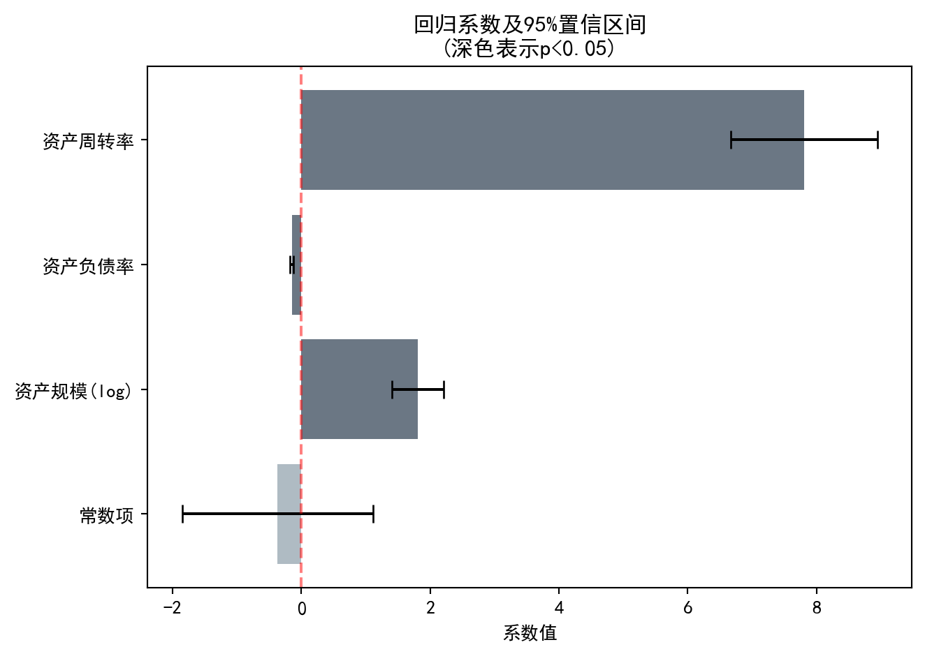
图 10.1 直观展示了各自变量的回归系数大小及其统计显著性。深色条形表示在5%水平下显著的变量,误差棒表示95%置信区间。下面通过 图 10.2 对比模型的预测值与实际值,评估模型拟合效果。
图 10.1 visually displays the magnitude of each independent variable’s regression coefficient and its statistical significance. Dark bars indicate variables significant at the 5% level, and error bars represent 95% confidence intervals. Next, we compare the model’s predicted values with actual values via 图 10.2 to assess the model fit.
# ========== 绘制实际值vs预测值散点图 ==========
# ========== Plot actual vs. predicted scatter plot ==========
predicted_roe_values_array = ols_regression_model.predict(independent_variables_dataframe)  # 计算预测值
                                                                                             # Calculate predicted values
matplot_figure, prediction_scatter_axes = plt.subplots(figsize=(7, 5))  # 创建单图画布
                                                                         # Create single-figure canvas
prediction_scatter_axes.scatter(dependent_variable_series, predicted_roe_values_array, alpha=0.5, color='#008080')  # 绘制散点图:实际值vs预测值
                                                                                                                     # Draw scatter plot: actual vs. predicted
prediction_scatter_axes.plot([dependent_variable_series.min(), dependent_variable_series.max()],  # 绘制45度完美预测线
                                                                                                   # Draw 45-degree perfect prediction line
    [dependent_variable_series.min(), dependent_variable_series.max()], 'r--', lw=2, label='完美预测线')  # 红色虚线标注完美预测基准
                                                                                                          # Red dashed line marking perfect prediction baseline
prediction_scatter_axes.set_xlabel('实际ROE (%)')   # X轴标签
                                                      # X-axis label
prediction_scatter_axes.set_ylabel('预测ROE (%)')   # Y轴标签
                                                      # Y-axis label
prediction_scatter_axes.set_title(f'实际 vs 预测 (R² = {ols_regression_model.rsquared:.3f})')  # 图标题含R²
                                                                                                 # Chart title with R²
prediction_scatter_axes.legend()                     # 显示图例
                                                      # Display legend
prediction_scatter_axes.grid(True, alpha=0.3)        # 添加网格线
                                                      # Add grid lines
plt.tight_layout()  # 自动调整子图间距
                     # Automatically adjust subplot spacing
plt.show()          # 显示图形
                     # Display the figure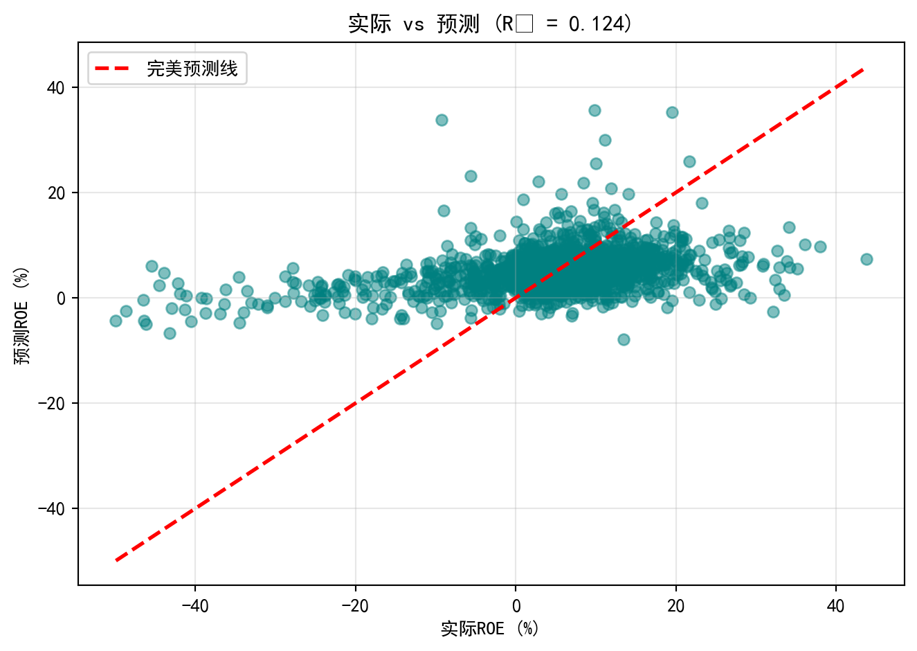
图 10.2 将模型预测的ROE与实际ROE进行对比。散点围绕红色45度”完美预测线”分布,但离散程度较大,尤其是在ROE极端值区域,预测偏差明显增大。这与\(R^2\)=0.124一致——模型捕捉了数据约12.4%的变异,但仍有近88%的ROE差异未被解释,提示现有三个财务变量远不能完整解释企业盈利能力的全貌,未来可考虑加入行业特征、公司治理等变量。
图 10.2 compares the model-predicted ROE with the actual ROE. The scatter points are distributed around the red 45-degree “perfect prediction line,” but the dispersion is substantial, especially in the extreme ROE regions where prediction errors increase noticeably. This is consistent with \(R^2\) = 0.124 — the model captures about 12.4% of the data variation, but nearly 88% of the ROE differences remain unexplained, suggesting that the current three financial variables are far from fully explaining the complete picture of corporate profitability. Future improvements could include adding industry characteristics, corporate governance variables, and other factors. ## 模型诊断 (Model Diagnostics) {#sec-diagnostics}
10.5.1 残差分析 (Residual Analysis)
残差分析是检验回归假设的核心工具(见 图 10.3)。
Residual analysis is the core tool for checking regression assumptions (see 图 10.3).
# ========== 残差诊断数据预处理 ==========
# ========== Residual Diagnostics Data Preprocessing ==========
model_residuals_array = ols_regression_model.resid                                      # 原始残差
# Raw residuals
fitted_values_array = ols_regression_model.fittedvalues                                  # 拟合值(预测值)
# Fitted values (predicted values)
standardized_residuals_array = ols_regression_model.get_influence().resid_studentized_internal  # 学生化残差
# Studentized residuals
from statsmodels.nonparametric.smoothers_lowess import lowess             # 导入LOWESS平滑方法
# Import LOWESS smoothing method
lowess_smoothing_result_array = lowess(np.sqrt(np.abs(standardized_residuals_array)), fitted_values_array, frac=0.6)  # 预计算平滑线
# Pre-compute smoothing line
normal_pdf_x_values = np.linspace(model_residuals_array.min() * 1.1, model_residuals_array.max() * 1.1, 100)  # 正态PDF的X轴范围
# X-axis range for the normal PDF
normal_pdf_y_values = stats.norm.pdf(normal_pdf_x_values, model_residuals_array.mean(), model_residuals_array.std())  # 正态PDF的Y值
# Y values of the normal PDF
残差和拟合值已计算完成。下面以四面板诊断图直观检查回归模型的各项基本假设:
Residuals and fitted values have been computed. The following four-panel diagnostic plots visually inspect the fundamental assumptions of the regression model:
# ========== 第1步:创建上排诊断图画布 ==========
# ========== Step 1: Create the upper-row diagnostic plot canvas ==========
matplot_figure, matplot_axes_top = plt.subplots(1, 2, figsize=(12, 5))  # 1行2列子图
# 1-row, 2-column subplots

# ========== 第2步:残差vs拟合值图(检验同方差性) ==========
# ========== Step 2: Residuals vs. Fitted Values plot (test homoscedasticity) ==========
residual_fitted_axes = matplot_axes_top[0]                               # 左侧子图
# Left subplot
residual_fitted_axes.scatter(fitted_values_array, model_residuals_array, alpha=0.5, color='#2C3E50')  # 绘制残差散点图
# Plot residual scatter points
residual_fitted_axes.axhline(y=0, color='red', linestyle='--')           # 添加零参考线
# Add zero reference line
residual_fitted_axes.set_xlabel('拟合值')                                 # X轴标签
# X-axis label
residual_fitted_axes.set_ylabel('残差')                                   # Y轴标签
# Y-axis label
residual_fitted_axes.set_title('残差 vs 拟合值\n(检验同方差性: 应无明显模式)')  # 图标题
# Plot title

# ========== 第3步:Q-Q图(检验残差正态性) ==========
# ========== Step 3: Q-Q Plot (test residual normality) ==========
qq_plot_axes = matplot_axes_top[1]                                       # 右侧子图
# Right subplot
stats.probplot(model_residuals_array, plot=qq_plot_axes)                  # 绘制正态概率图
# Plot normal probability plot
qq_plot_axes.set_title('正态Q-Q图\n(检验正态性: 点应落在直线上)')          # 图标题
# Plot title

plt.tight_layout()  # 自动调整子图间距
# Automatically adjust subplot spacing
plt.show()          # 显示图形
# Display the figure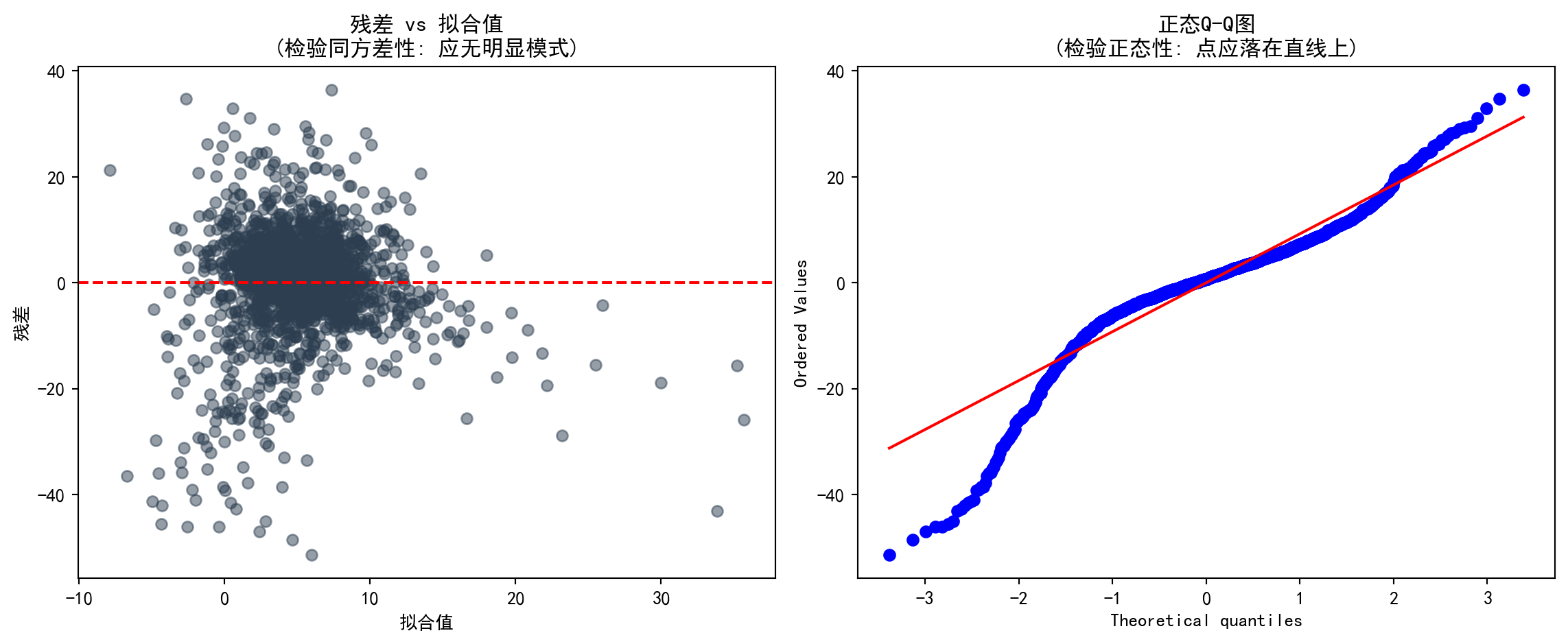
图 10.3 中,上排两图分别检验同方差性和正态性假设。残差vs拟合值图中,若残差随拟合值呈扇形散开,则提示存在异方差;Q-Q图中,点偏离直线越远,正态性假设越可疑。下面通过 图 10.4 绘制Scale-Location图和残差分布直方图,进一步验证方差稳定性和分布形态。
In 图 10.3, the two upper-row plots test the homoscedasticity and normality assumptions, respectively. In the residuals vs. fitted values plot, if the residuals fan out as fitted values increase, it suggests heteroscedasticity; in the Q-Q plot, the farther the points deviate from the straight line, the more questionable the normality assumption. Below, 图 10.4 presents the Scale-Location plot and residual histogram to further verify variance stability and distributional shape.
# ========== 第1步:创建下排诊断图画布 ==========
# ========== Step 1: Create the lower-row diagnostic plot canvas ==========
matplot_figure, matplot_axes_bottom = plt.subplots(1, 2, figsize=(12, 5))  # 1行2列子图
# 1-row, 2-column subplots

# ========== 第2步:Scale-Location图(另一种同方差性检验) ==========
# ========== Step 2: Scale-Location plot (another homoscedasticity test) ==========
scale_location_axes = matplot_axes_bottom[0]                             # 左侧子图
# Left subplot
scale_location_axes.scatter(fitted_values_array,                         # 横轴为拟合值
    np.sqrt(np.abs(standardized_residuals_array)),                        # 纵轴为标准化残差绝对值的平方根
    alpha=0.5, color='#008080')                                          # 设置透明度和颜色
# X-axis: fitted values; Y-axis: square root of absolute standardized residuals; set transparency and color
scale_location_axes.set_xlabel('拟合值')                                  # X轴标签
# X-axis label
scale_location_axes.set_ylabel('√|标准化残差|')                           # Y轴标签
# Y-axis label
scale_location_axes.set_title('Scale-Location图\n(红线应水平)')            # 图标题
# Plot title
scale_location_axes.plot(lowess_smoothing_result_array[:, 0], lowess_smoothing_result_array[:, 1], 'r-', lw=2)  # 绘制LOWESS红色平滑线
# Plot the LOWESS red smoothing line

# ========== 第3步:残差直方图(检验残差分布形态) ==========
# ========== Step 3: Residual histogram (test residual distribution shape) ==========
residual_histogram_axes = matplot_axes_bottom[1]                         # 右侧子图
# Right subplot
residual_histogram_axes.hist(model_residuals_array, bins=30, density=True, alpha=0.7, color='#F0A700')  # 残差频率直方图
# Residual frequency histogram
residual_histogram_axes.plot(normal_pdf_x_values, normal_pdf_y_values, 'r-', lw=2, label='正态分布')  # 叠加理论正态分布密度曲线
# Overlay theoretical normal distribution density curve
residual_histogram_axes.set_xlabel('残差')                                # X轴标签
# X-axis label
residual_histogram_axes.set_ylabel('密度')                                # Y轴标签
# Y-axis label
residual_histogram_axes.set_title('残差分布\n(应接近正态分布)')             # 图标题
# Plot title
residual_histogram_axes.legend()                                          # 显示图例
# Display legend

plt.tight_layout()  # 自动调整子图间距
# Automatically adjust subplot spacing
plt.show()          # 显示图形
# Display the figure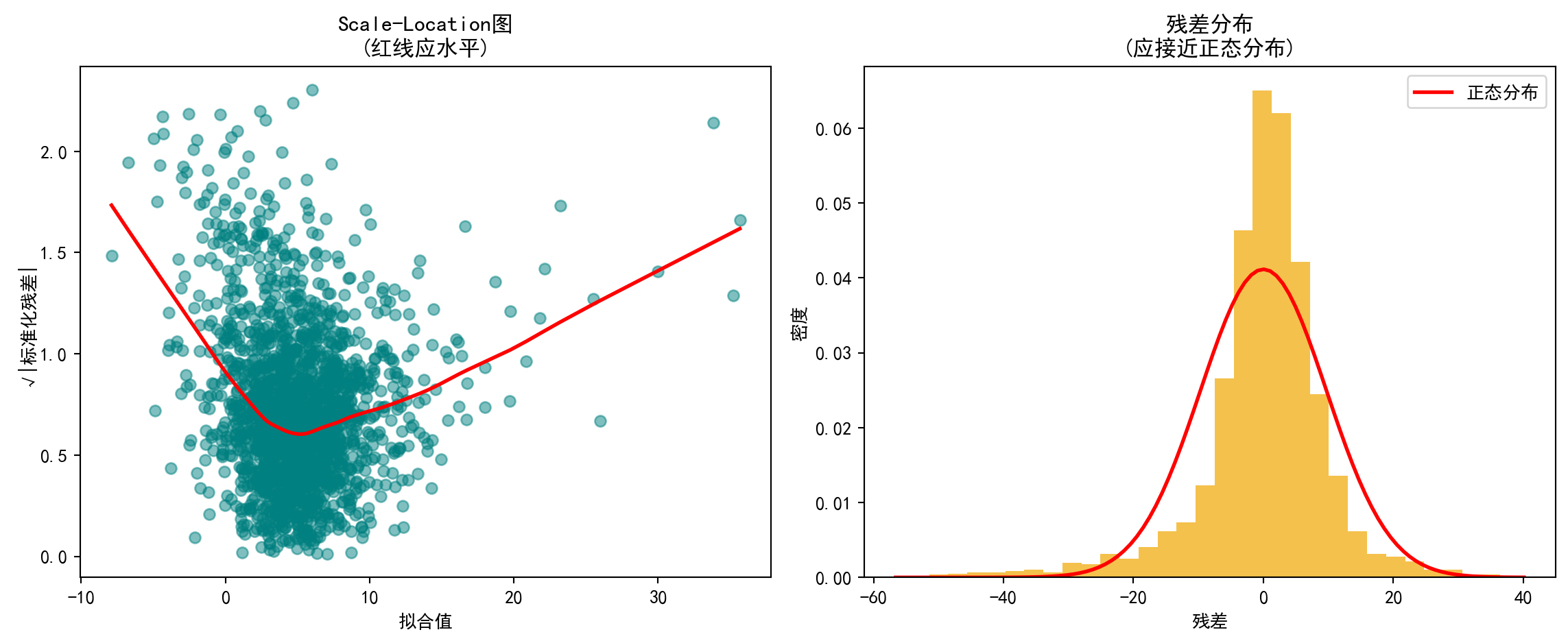
图 10.4 中,左图(Scale-Location)显示LOWESS平滑线并非水平,随拟合值增大呈上升趋势,初步提示残差方差并不恒定,存在异方差嫌疑。右图(残差直方图)显示残差分布大致呈钟形但存在尖峰和厚尾特征,与正态分布红线有一定偏差,表明残差正态性假设仅近似成立。为进一步量化异方差性,下面进行正式的统计检验。
In 图 10.4, the left panel (Scale-Location) shows that the LOWESS smoothing line is not horizontal but trends upward as fitted values increase, providing preliminary evidence that residual variance is not constant—suggesting heteroscedasticity. The right panel (residual histogram) shows that the residual distribution is roughly bell-shaped but exhibits excess kurtosis and heavy tails, deviating somewhat from the red normal distribution curve, indicating that the normality assumption holds only approximately. To further quantify heteroscedasticity, we proceed with formal statistical tests below.
10.5.2 异方差检验 (Heteroscedasticity Tests)
异方差检验结果如 表 10.4 所示。
The heteroscedasticity test results are shown in 表 10.4.
# ========== 导入异方差检验函数 ==========
# ========== Import heteroscedasticity test functions ==========
from statsmodels.stats.diagnostic import het_breuschpagan, het_white  # Breusch-Pagan和White检验
# Breusch-Pagan and White tests

# ========== 第1步:Breusch-Pagan检验 ==========
# ========== Step 1: Breusch-Pagan test ==========
breusch_pagan_statistic, breusch_pagan_p_value, _, _ = het_breuschpagan(  # 执行BP检验
    ols_regression_model.resid, ols_regression_model.model.exog)          # 输入残差和设计矩阵
# Execute BP test with residuals and design matrix as inputs

# ========== 第2步:White检验 ==========
# ========== Step 2: White test ==========
white_test_statistic, white_test_p_value, _, _ = het_white(               # 执行White检验
    ols_regression_model.resid, ols_regression_model.model.exog)          # 输入残差和设计矩阵
# Execute White test with residuals and design matrix as inputs
Breusch-Pagan检验与White检验执行完毕。下面输出检验结果并根据异方差情况选择稳健标准误。
The Breusch-Pagan test and White test have been completed. Below we output the test results and choose robust standard errors based on the heteroscedasticity findings.
# ========== 第3步:输出检验结果与结论 ==========
# ========== Step 3: Output test results and conclusions ==========
print('=== 异方差性检验 ===\n')  # 输出异方差检验的分隔标题
# Print header for heteroscedasticity tests
print('1. Breusch-Pagan检验:')                                       # 原假设:同方差
# Null hypothesis: homoscedasticity
print(f'   LM统计量 = {breusch_pagan_statistic:.4f}')              # LM检验统计量
# LM test statistic
print(f'   p值 = {breusch_pagan_p_value:.4f}')                            # p值
# p-value
print(f'   结论: {"存在异方差" if breusch_pagan_p_value < 0.05 else "不能拒绝同方差假设"}')  # 根据BP检验p值输出结论
# Output conclusion based on BP test p-value

print('\n2. White检验:')                                              # White检验(更全面,包含交叉项)
# White test (more comprehensive, includes cross terms)
print(f'   LM统计量 = {white_test_statistic:.4f}')                 # LM检验统计量
# LM test statistic
print(f'   p值 = {white_test_p_value:.4f}')                               # p值
# p-value
print(f'   结论: {"存在异方差" if white_test_p_value < 0.05 else "不能拒绝同方差假设"}')  # 根据White检验p值输出结论
# Output conclusion based on White test p-value

# ========== 第4步:若存在异方差则使用稳健标准误 ==========
# ========== Step 4: Use robust standard errors if heteroscedasticity is present ==========
if breusch_pagan_p_value < 0.05 or white_test_p_value < 0.05:              # 任一检验拒绝同方差
    # If either test rejects homoscedasticity
    print('\n建议: 使用稳健标准误(Robust Standard Errors)')       # 输出建议
    # Print recommendation
    robust_standard_errors_model = ols_regression_model.get_robustcov_results(cov_type='HC3')  # HC3稳健标准误
    # HC3 robust standard errors
    print('\n稳健标准误下的结果:')                                   # 显示标题
    # Display heading
    print(robust_standard_errors_model.summary().tables[1])                 # 输出稳健回归结果表
    # Output robust regression results table
=== 异方差性检验 ===
1. Breusch-Pagan检验:
LM统计量 = 197.4681
p值 = 0.0000
结论: 存在异方差
2. White检验:
LM统计量 = 405.7861
p值 = 0.0000
结论: 存在异方差
建议: 使用稳健标准误(Robust Standard Errors)
稳健标准误下的结果:
==================================================================================
coef std err t P>|t| [0.025 0.975]
----------------------------------------------------------------------------------
const -0.3667 0.875 -0.419 0.675 -2.083 1.349
log_assets 1.8094 0.278 6.507 0.000 1.264 2.355
debt_ratio -0.1494 0.020 -7.412 0.000 -0.189 -0.110
asset_turnover 7.8025 1.050 7.430 0.000 5.743 9.862
==================================================================================表 10.4 结果明确:Breusch-Pagan检验(LM=197.47,p<0.001)和White检验(LM=405.79,p<0.001)均强烈拒绝同方差原假设,确认模型存在显著的异方差性。鉴于此,我们采用HC3稳健标准误进行推断。在稳健标准误下,三个自变量的系数估计值不变,但标准误普遍增大(尤其是asset_turnover的标准误从0.517增至1.050),不过所有变量仍在1%水平下显著,表明异方差性虽然影响了标准误的精度,但并未改变我们关于变量显著性的基本结论。
The results in 表 10.4 are clear: the Breusch-Pagan test (LM=197.47, p<0.001) and the White test (LM=405.79, p<0.001) both strongly reject the null hypothesis of homoscedasticity, confirming the presence of significant heteroscedasticity in the model. Accordingly, we adopt HC3 robust standard errors for inference. Under robust standard errors, the coefficient estimates for all three independent variables remain unchanged, but the standard errors are generally larger (notably, the standard error of asset_turnover increases from 0.517 to 1.050). Nevertheless, all variables remain significant at the 1% level, indicating that while heteroscedasticity affects the precision of standard errors, it does not alter our fundamental conclusions regarding variable significance.
10.5.3 多重共线性诊断 (Multicollinearity Diagnostics)
方差膨胀因子(VIF)用于检测多重共线性:
The Variance Inflation Factor (VIF) is used to detect multicollinearity:
\[ VIF_j = \frac{1}{1-R_j^2} \]
其中\(R_j^2\)是变量\(X_j\)对其他自变量回归的\(R^2\)。
where \(R_j^2\) is the \(R^2\) from regressing variable \(X_j\) on all other independent variables.
VIF 诊断结果如 表 10.5 所示。
The VIF diagnostic results are shown in 表 10.5.
# ========== 导入VIF计算函数 ==========
# ========== Import VIF computation function ==========
from statsmodels.stats.outliers_influence import variance_inflation_factor  # 方差膨胀因子
# Variance Inflation Factor

# ========== 第1步:计算各自变量的VIF ==========
# ========== Step 1: Compute VIF for each independent variable ==========
vif_independent_variables_dataframe = multivariate_analysis_dataframe[['log_assets', 'debt_ratio', 'asset_turnover']]  # 提取自变量
# Extract independent variables
vif_results_dataframe = pd.DataFrame()                                     # 创建结果DataFrame
# Create results DataFrame
vif_results_dataframe['变量'] = vif_independent_variables_dataframe.columns    # 变量名列
# Variable name column
vif_results_dataframe['VIF'] = [variance_inflation_factor(                  # 计算每个变量的VIF
    vif_independent_variables_dataframe.values, i)  # 传入自变量矩阵和当前变量索引
    for i in range(vif_independent_variables_dataframe.shape[1])]           # 遍历所有自变量
# Compute VIF for each variable by passing the variable matrix and current variable index, iterating over all independent variables
各自变量的方差膨胀因子(VIF)计算完毕。下面输出诊断结果并给出多重共线性的判断结论。
The Variance Inflation Factors (VIF) for all independent variables have been computed. Below we output the diagnostic results and provide conclusions regarding multicollinearity.
# ========== 第2步:输出VIF结果与判断标准 ==========
# ========== Step 2: Output VIF results and decision criteria ==========
print('=== 多重共线性诊断 (VIF) ===\n')  # 输出VIF诊断的分隔标题
# Print header for VIF diagnostics
print(vif_results_dataframe.to_string(index=False))  # 打印VIF表格
# Print VIF table

print('\n判断标准:')                    # VIF解读规则
# Decision criteria
print('- VIF < 5: 无多重共线性问题')     # 安全范围
# VIF < 5: No multicollinearity issue
print('- 5 ≤ VIF < 10: 轻度多重共线性')   # 警告范围
# 5 ≤ VIF < 10: Mild multicollinearity
print('- VIF ≥ 10: 严重多重共线性,需处理')  # 危险范围
# VIF ≥ 10: Severe multicollinearity, action required

# ========== 第3步:输出诊断结论 ==========
# ========== Step 3: Output diagnostic conclusion ==========
maximum_vif_value = vif_results_dataframe['VIF'].max()  # 找出最大VIF值
# Find the maximum VIF value
if maximum_vif_value < 5:                               # VIF<5:无问题
    # VIF < 5: No issue
    print(f'\n结论: 最大VIF = {maximum_vif_value:.2f} < 5,不存在多重共线性问题')  # 输出无多重共线性的结论
    # Output conclusion: no multicollinearity
elif maximum_vif_value < 10:                             # 5≤VIF<10:轻度问题
    # 5 ≤ VIF < 10: Mild issue
    print(f'\n结论: 最大VIF = {maximum_vif_value:.2f},存在轻度多重共线性')  # 输出轻度多重共线性的结论
    # Output conclusion: mild multicollinearity
else:                                                   # VIF≥10:严重问题
    # VIF ≥ 10: Severe issue
    print(f'\n结论: 最大VIF = {maximum_vif_value:.2f} ≥ 10,存在严重多重共线性,建议删除或合并变量')  # 输出严重多重共线性的结论和建议
    # Output conclusion: severe multicollinearity; recommend removing or merging variables
=== 多重共线性诊断 (VIF) ===
变量 VIF
log_assets 6.795510
debt_ratio 6.696457
asset_turnover 2.875645
判断标准:
- VIF < 5: 无多重共线性问题
- 5 ≤ VIF < 10: 轻度多重共线性
- VIF ≥ 10: 严重多重共线性,需处理
结论: 最大VIF = 6.80,存在轻度多重共线性表 10.5 显示,log_assets(VIF=6.80)和debt_ratio(VIF=6.70)的方差膨胀因子处于5-10的”轻度多重共线性”区间,而asset_turnover(VIF=2.88)无多重共线性问题。这一结果符合经济直觉:资产规模较大的企业通常也具有更高的举债能力,导致两者相关性较高。但由于所有VIF均低于10的严重阈值,参数估计的可靠性尚可接受,暂无需删除或合并变量。
表 10.5 shows that the VIFs for log_assets (VIF=6.80) and debt_ratio (VIF=6.70) fall within the 5–10 “mild multicollinearity” range, while asset_turnover (VIF=2.88) has no multicollinearity issue. This result is consistent with economic intuition: larger firms typically have greater borrowing capacity, leading to higher correlation between the two. However, since all VIFs are below the severe threshold of 10, the reliability of the parameter estimates remains acceptable, and there is no immediate need to remove or merge variables.
10.6 从理论到实践:苦活累活 (From Theory to Practice: The “Dirty Work”)
10.6.1 逐步回归的陷阱 (The Stepwise Trap)
在计算机算力过剩的今天,很多分析师喜欢把几十个变量扔进软件,点击”Stepwise Regression”(逐步回归),让算法自动筛选出”显著”的变量。
In today’s era of abundant computing power, many analysts like to throw dozens of variables into software, click “Stepwise Regression,” and let the algorithm automatically select “significant” variables.
为什么这是统计学之罪:
- R2 虚高:算法通过”数据挖掘”强行拟合噪声。
- 系数有偏:选出来的变量系数绝对值往往被高估(Winner’s Curse)。
- 推断失效:标准的 t 检验和 p 值假设你的模型是预先设定的,而不是”看数据下菜碟”选出来的。
Why this is a statistical sin:
- Inflated R²: The algorithm force-fits noise through “data mining.”
- Biased coefficients: The absolute values of selected variable coefficients tend to be overestimated (Winner’s Curse).
- Invalid inference: Standard t-tests and p-values assume your model was pre-specified, not cherry-picked from the data.
对策:使用 Lasso / Ridge 正则化回归,或者基于领域知识(Domain Knowledge)和因果图(DAG)手工选择变量。
Countermeasures: Use Lasso / Ridge regularized regression, or manually select variables based on domain knowledge and causal diagrams (DAGs).
10.6.2 表2谬误 (Table 2 Fallacy)
在一篇论文中(通常表1是描述性统计,表2是主回归结果),我们往往会看到一个因变量 \(Y\) 和多个自变量 \(X_1, X_2, \dots\)。
In an academic paper (where Table 1 is typically descriptive statistics and Table 2 is the main regression results), we often see one dependent variable \(Y\) and multiple independent variables \(X_1, X_2, \dots\).
谬误:读者(甚至作者)倾向于认为表中的每一个系数 \(\beta_i\) 都有因果解释。
真相:在同一个模型中,不同的变量角色不同。有些是我们要研究的因果变量(Treatment),有些只是为了消除偏差的混淆变量(Confounder)。
The fallacy: Readers (and even authors) tend to interpret every coefficient \(\beta_i\) in the table as having a causal interpretation.
The truth: Within the same model, different variables play different roles. Some are the treatment variables we wish to study causally, while others are merely confounders included to eliminate bias.
混淆变量的系数通常是没有因果解释的,它们只是为了让因果变量的估计更准确而存在的”配角”。
The coefficients of confounders typically have no causal interpretation—they are merely “supporting actors” included to make the causal variable estimates more accurate.
10.7 变量选择 (Variable Selection)
10.7.1 信息准则 (Information Criteria)
在变量选择中,我们面临一个核心矛盾:模型拟合度 vs. 模型复杂度。加入更多变量总能提高 \(R^2\)(至少不会降低),但过于复杂的模型会拟合噪声(过拟合),在预测新数据时表现反而更差。信息准则正是为了解决这个矛盾而设计的——它们在衡量模型对数据拟合程度的同时,对模型的参数个数施加”惩罚”,从而在拟合优度和模型简约性之间取得平衡。
In variable selection, we face a core trade-off: model fit vs. model complexity. Adding more variables always increases \(R^2\) (or at least does not decrease it), but an overly complex model will fit noise (overfitting) and perform worse when predicting new data. Information criteria are designed to resolve this trade-off—they measure how well the model fits the data while imposing a “penalty” on the number of parameters, thus striking a balance between goodness of fit and model parsimony.
信息准则的核心思想是:好的模型应该用尽可能少的参数来解释尽可能多的数据变异。在比较多个候选模型时,我们选择信息准则值最小的模型作为最优模型。
The core idea behind information criteria is: a good model should explain as much data variation as possible with as few parameters as possible. When comparing multiple candidate models, we select the model with the smallest information criterion value as the optimal model.
AIC (Akaike Information Criterion)(式 10.10):
\[ AIC = n \ln\left(\frac{RSS}{n}\right) + 2(p+1) \tag{10.10}\]
AIC由日本统计学家赤池弘次(Hirotugu Akaike)于1974年提出。公式中第一项 \(n\ln(RSS/n)\) 反映模型的拟合程度(RSS越小,拟合越好,该项越小),第二项 \(2(p+1)\) 是对参数个数的惩罚(每多一个参数,AIC增加2)。AIC的理论基础是Kullback-Leibler信息量,它度量的是候选模型与”真实模型”之间的距离。
AIC was proposed by the Japanese statistician Hirotugu Akaike in 1974. In the formula, the first term \(n\ln(RSS/n)\) reflects the model’s goodness of fit (the smaller the RSS, the better the fit, and the smaller this term), while the second term \(2(p+1)\) penalizes the number of parameters (each additional parameter increases AIC by 2). The theoretical foundation of AIC is the Kullback-Leibler divergence, which measures the distance between the candidate model and the “true model.”
BIC (Bayesian Information Criterion)(式 10.11):
\[ BIC = n \ln\left(\frac{RSS}{n}\right) + (p+1)\ln(n) \tag{10.11}\]
BIC(也称Schwarz准则)的结构与AIC类似,但惩罚项为 \((p+1)\ln(n)\)。由于当样本量 \(n > 7\) 时 \(\ln(n) > 2\),BIC对参数个数的惩罚比AIC更重,因此BIC倾向于选择更简约的模型。在实践中,如果AIC和BIC选出不同的模型,BIC选出的模型通常变量更少。
BIC (also known as the Schwarz criterion) has a structure similar to AIC, but with a penalty term of \((p+1)\ln(n)\). Since \(\ln(n) > 2\) when the sample size \(n > 7\), BIC penalizes the number of parameters more heavily than AIC, and therefore BIC tends to select more parsimonious models. In practice, if AIC and BIC select different models, the BIC-selected model typically has fewer variables.
不同变量组合的模型比较结果如 表 10.6 所示。
The model comparison results for different variable combinations are shown in 表 10.6.
# ========== 导入组合函数 ==========
# ========== Import combinations function ==========
# 比较不同变量组合的模型
# Compare models with different variable combinations
from itertools import combinations  # 生成变量的所有子集组合
# Generate all subset combinations of variables

# ========== 第1步:枚举所有自变量组合并逐一建模 ==========
# ========== Step 1: Enumerate all variable combinations and fit models one by one ==========
candidate_variables_list = ['log_assets', 'debt_ratio', 'asset_turnover']  # 候选自变量列表
# List of candidate independent variables
model_comparison_results_list = []  # 存储各模型评估结果
# Store evaluation results for each model

for r in range(1, len(candidate_variables_list) + 1):  # 遍历变量数1到3
    # Iterate over variable counts from 1 to 3
    for combo in combinations(candidate_variables_list, r):  # 枚举当前变量数下的所有组合
        # Enumerate all combinations for the current variable count
        temporary_independent_variables_dataframe = sm.add_constant(  # 添加截距项
            multivariate_analysis_dataframe[list(combo)])  # 提取当前组合的自变量
        # Add intercept and extract independent variables for current combination
        temporary_regression_model = sm.OLS(  # OLS回归拟合
            dependent_variable_series, temporary_independent_variables_dataframe).fit()  # 传入因变量和自变量矩阵并拟合模型
        # Fit OLS regression with dependent and independent variable matrices
        model_comparison_results_list.append({  # 记录模型评估指标
            '变量': ' + '.join(combo),                           # 变量组合名称
            'R²': temporary_regression_model.rsquared,           # 决定系数
            '调整R²': temporary_regression_model.rsquared_adj,   # 调整后决定系数
            'AIC': temporary_regression_model.aic,               # 赤池信息准则(越小越好)
            'BIC': temporary_regression_model.bic                # 贝叶斯信息准则(越小越好)
        })
        # Record model evaluation metrics: variable combination, R², adjusted R², AIC, BIC

model_comparison_results_dataframe = pd.DataFrame(model_comparison_results_list)  # 转为DataFrame
# Convert to DataFrame
各变量组合模型拟合完毕。下面输出模型比较结果并标记最优模型。
All variable combination models have been fitted. Below we output the model comparison results and identify the optimal model.
print('=== 模型比较 ===\n')  # 输出模型比较的分隔标题
# Print header for model comparison
print(model_comparison_results_dataframe.round(4).to_string(index=False))  # 输出模型对比表
# Print model comparison table

# ========== 第2步:标记最佳模型并输出结论 ==========
# ========== Step 2: Identify the best model and output conclusions ==========
best_aic_model_series = model_comparison_results_dataframe.loc[  # AIC最小的模型
    model_comparison_results_dataframe['AIC'].idxmin()]  # 查找AIC最小值所在行的索引
# Locate the model with the smallest AIC
best_bic_model_series = model_comparison_results_dataframe.loc[  # BIC最小的模型
    model_comparison_results_dataframe['BIC'].idxmin()]  # 查找BIC最小值所在行的索引
# Locate the model with the smallest BIC

print(f'\n根据AIC, 最优模型: {best_aic_model_series["变量"]}')  # 输出AIC最优模型
# Output the optimal model according to AIC
print(f'根据BIC, 最优模型: {best_bic_model_series["变量"]}')    # 输出BIC最优模型
# Output the optimal model according to BIC
=== 模型比较 ===
变量 R² 调整R² AIC BIC
log_assets 0.0086 0.0081 14546.5514 14557.6903
debt_ratio 0.0120 0.0115 14539.8192 14550.9581
asset_turnover 0.0596 0.0591 14444.1378 14455.2766
log_assets + debt_ratio 0.0417 0.0407 14482.6920 14499.4002
log_assets + asset_turnover 0.0651 0.0642 14434.7379 14451.4462
debt_ratio + asset_turnover 0.0888 0.0879 14385.0008 14401.7090
log_assets + debt_ratio + asset_turnover 0.1235 0.1222 14311.7633 14334.0409
根据AIC, 最优模型: log_assets + debt_ratio + asset_turnover
根据BIC, 最优模型: log_assets + debt_ratio + asset_turnover表 10.6 对3个候选变量的所有7种组合进行了系统比较。结果显示,AIC和BIC一致选出包含全部三个变量的模型(log_assets + debt_ratio + asset_turnover)为最优:该模型的AIC=14311.76和BIC=14334.04均为所有候选模型中最低,\(R^2\)=0.1235也最高。这验证了我们早期基于经济理论选择的变量集合是恰当的——三个维度(规模、杠杆、运营效率)缺一不可。
表 10.6 systematically compares all 7 combinations of the 3 candidate variables. The results show that both AIC and BIC unanimously select the full three-variable model (log_assets + debt_ratio + asset_turnover) as optimal: this model has the lowest AIC=14311.76 and BIC=14334.04 among all candidates, and also the highest \(R^2\)=0.1235. This validates that the variable set we chose earlier based on economic theory is appropriate—the three dimensions (scale, leverage, and operating efficiency) are all indispensable.
10.7.2 “厨房水槽”陷阱 (Kitchen Sink Regression)
新手常犯的一个错误是:把所有能找到的变量都扔进回归模型里,以为这样就能控制更多因素。 这被称为”厨房水槽”回归(Everything but the kitchen sink)。
A common mistake made by beginners is: throwing every available variable into the regression model, believing this will control for more factors. This is known as “kitchen sink” regression (Everything but the kitchen sink).
为什么这是危险的?
Why is this dangerous?
多重共线性:变量越多,共线性风险越高,参数估计方差膨胀,变得极不稳定。
伪相关:在大样本和多变量下,纯随机变量也可能显著(p-hacking风险)。
对撞机偏差(Collider Bias):如果不小心控制了”结果的共同结果”(Collider),反而会制造出原本不存在的伪相关。例如,为了研究”智商”对”成功”的影响,控制了”是否常春藤毕业”,可能会发现智商越高越不成功(因为能进常春藤的,要么极聪明,要么极努力/有背景。控制了常春藤,就在聪明和努力之间制造了负相关)。
Multicollinearity: The more variables included, the higher the risk of collinearity—parameter estimate variances inflate and become extremely unstable.
Spurious correlations: With large samples and many variables, even purely random variables may appear significant (p-hacking risk).
Collider bias: If you inadvertently control for a “common outcome of outcomes” (a collider), you may actually create spurious correlations that did not originally exist. For example, when studying the effect of “IQ” on “success,” controlling for “Ivy League graduation” might lead to the finding that higher IQ is associated with less success (because those who get into the Ivy League are either extremely smart or extremely hardworking/well-connected; controlling for Ivy League status creates a negative correlation between intelligence and effort).
原则:变量选择应基于因果图(DAG)和领域知识,而不是盲目追求高 \(R^2\)。只有混淆变量(Confounder)需要控制,中介变量(Mediator)和对撞机(Collider)通常不应控制。
Principle: Variable selection should be based on causal diagrams (DAGs) and domain knowledge, rather than blindly pursuing a high \(R^2\). Only confounders need to be controlled for; mediators and colliders generally should not be controlled for. ## 启发式思考题 (Heuristic Problems) {#sec-heuristic-problems-ch10}
1. 辛普森悖论 (Simpson’s Paradox) 的回归版 - 实验:生成一个数据集,使得 \(Y\) 和 \(X_1\) 在单变量回归中呈正相关 (\(r > 0\))。 - 操作:加入一个混淆变量 \(X_2\)(例如性别、分组),使得在多元回归中 \(X_1\) 的系数变为负数 (\(\beta_1 < 0\))。 - 反思:如果不加控制变量,我们可能会得到完全相反的结论。这就是为什么”看平均值”(单变量)经常会骗人。
1. Regression Version of Simpson’s Paradox - Experiment: Generate a dataset where \(Y\) and \(X_1\) are positively correlated in a univariate regression (\(r > 0\)). - Task: Introduce a confounding variable \(X_2\) (e.g., gender, group membership) such that in a multiple regression, the coefficient of \(X_1\) becomes negative (\(\beta_1 < 0\)). - Reflection: Without controlling for confounders, we may reach a completely opposite conclusion. This is why “just looking at averages” (univariate analysis) can often be misleading.
辛普森悖论代码演示
Simpson’s Paradox Code Demonstration
# ========== 导入所需库 ==========
# ========== Import required libraries ==========
import numpy as np                  # 数值计算
                                    # Numerical computation
import pandas as pd                 # 数据处理
                                    # Data manipulation
import statsmodels.api as sm        # 统计建模
                                    # Statistical modeling
import matplotlib.pyplot as plt     # 数据可视化
                                    # Data visualization

# ========== 第1步:设置随机种子并构造分组数据 ==========
# ========== Step 1: Set random seed and construct grouped data ==========
np.random.seed(42)                  # 固定随机种子保证可重复
                                    # Fix random seed for reproducibility
n_per_group = 100                   # 每组样本量
                                    # Sample size per group

# 构造两组数据:组内X1与Y负相关,但组间均值差异造成整体正相关假象
# Construct two groups: X1 and Y are negatively correlated within each group, but between-group mean differences create a spurious overall positive correlation
# 组0:X1均值低,Y均值低
# Group 0: Low mean of X1, low mean of Y
x1_group_0 = np.random.normal(2, 1, n_per_group)                             # X1 ~ N(2, 1)
y_group_0 = -0.5 * x1_group_0 + np.random.normal(0, 1, n_per_group) + 5     # 组内斜率为-0.5(负相关)
                                                                              # Within-group slope is -0.5 (negative correlation)

# 组1:X1均值高,Y均值高
# Group 1: High mean of X1, high mean of Y
x1_group_1 = np.random.normal(5, 1, n_per_group)                             # X1 ~ N(5, 1)
y_group_1 = -0.5 * x1_group_1 + np.random.normal(0, 1, n_per_group) + 15    # 组内斜率为-0.5(负相关)
                                                                              # Within-group slope is -0.5 (negative correlation)
辛普森悖论模拟数据构造完毕。下面合并数据并分别进行简单回归与多元回归。
The simulated data for demonstrating Simpson’s Paradox has been constructed. Next, we merge the data and perform both simple regression and multiple regression.
# ========== 第2步:合并数据并分别回归 ==========
# ========== Step 2: Merge data and run separate regressions ==========
x1_combined_array = np.concatenate([x1_group_0, x1_group_1])       # 合并X1
                                                                    # Concatenate X1 from both groups
y_combined_array = np.concatenate([y_group_0, y_group_1])           # 合并Y
                                                                    # Concatenate Y from both groups
group_indicator_array = np.repeat([0, 1], n_per_group)              # 组别标识(0或1)
                                                                    # Group indicator (0 or 1)

# 不控制组别的简单回归:遗漏了组别这个关键混淆变量
# Simple regression without controlling for group: omitting the key confounding variable
simple_design_matrix = sm.add_constant(x1_combined_array)           # 仅用X1作为自变量(遗漏组别)
                                                                    # Use only X1 as the predictor (group omitted)
simple_regression_model = sm.OLS(y_combined_array, simple_design_matrix).fit()  # 简单OLS拟合(估计结果存在遗漏变量偏误)
                                                                                # Simple OLS fit (estimates suffer from omitted variable bias)

# 控制组别的多元回归:加入组别虚拟变量消除混淆
# Multiple regression controlling for group: add group dummy variable to eliminate confounding
multiple_design_dataframe = pd.DataFrame({                          # 构建包含组别虚拟变量的设计矩阵
                                                                    # Build design matrix with group dummy variable
    'x1': x1_combined_array,                                        # 自变量X1(包含信号和噪声)
                                                                    # Predictor X1 (contains both signal and noise)
    'group': group_indicator_array                                   # 组别虚拟变量(控制组间均值差异)
                                                                    # Group dummy variable (controls between-group mean differences)
})
multiple_design_matrix = sm.add_constant(multiple_design_dataframe)  # 添加截距项构成完整设计矩阵
                                                                     # Add intercept to form the complete design matrix
multiple_regression_model = sm.OLS(y_combined_array, multiple_design_matrix).fit()  # 多元OLS拟合(消除了组别混淆后的估计)
                                                                                    # Multiple OLS fit (estimates after removing group confounding)
数据构造与回归模型拟合完成。下面输出对比结果并绘制可视化图。
Data construction and regression model fitting are complete. Next, we output the comparison results and create visualizations.
# ========== 第3步:输出回归结果对比 ==========
# ========== Step 3: Output regression result comparison ==========
print('=== 辛普森悖论演示 ===')  # 输出辛普森悖论演示的分隔标题
                                 # Print section header for Simpson's Paradox demonstration
print(f'简单回归 (不控制组别): X1 系数 = {simple_regression_model.params[1]:.4f} (正相关!)')     # 不控制混淆变量时X1系数为正(虚假正相关)
                                                                                                  # X1 coefficient is positive without controlling for confounders (spurious positive correlation)
print(f'多元回归 (控制组别):   X1 系数 = {multiple_regression_model.params["x1"]:.4f} (负相关!)')  # 控制组别后X1系数翻转为负(揭示真实负相关)
                                                                                                    # X1 coefficient flips to negative after controlling for group (reveals true negative correlation)
print(f'                       group 系数 = {multiple_regression_model.params["group"]:.4f}')      # 组间均值差异(混淆变量的效应)
                                                                                                    # Between-group mean difference (effect of the confounding variable)
=== 辛普森悖论演示 ===
简单回归 (不控制组别): X1 系数 = 1.7655 (正相关!)
多元回归 (控制组别): X1 系数 = -0.5592 (负相关!)
group 系数 = 10.2721回归结果惊人地展示了辛普森悖论:在不控制组别的简单回归中,\(X_1\)的系数为+1.7655,暗示\(X_1\)与\(Y\)正相关;然而,一旦在多元回归中加入组别虚拟变量,\(X_1\)的系数翻转为-0.5592,揭示了\(X_1\)与\(Y\)的真实关系其实是负相关。组别效应高达10.2721,这个被遗漏的混淆变量造成了完全相反的结论。下面绘制双面板散点图,直观展示这一惊人的翻转现象。
The regression results strikingly demonstrate Simpson’s Paradox: in the simple regression without controlling for group, the coefficient of \(X_1\) is +1.7655, suggesting a positive correlation between \(X_1\) and \(Y\); however, once the group dummy variable is added in the multiple regression, the coefficient of \(X_1\) flips to -0.5592, revealing that the true relationship between \(X_1\) and \(Y\) is actually negative. The group effect is as large as 10.2721—this omitted confounding variable led to a completely opposite conclusion. Below, we create a dual-panel scatter plot to visually illustrate this striking reversal.
# ========== 第4步:可视化——双面板对比 ==========
# ========== Step 4: Visualization — dual-panel comparison ==========
matplot_figure, matplot_axes_array = plt.subplots(1, 2, figsize=(14, 5))  # 创建1行2列子图
                                                                          # Create 1×2 subplot layout

# 左图:不区分组别(显示虚假的正相关)
# Left panel: Without distinguishing groups (shows spurious positive correlation)
overall_scatter_axes = matplot_axes_array[0]                               # 左子图
                                                                           # Left subplot
overall_scatter_axes.scatter(x1_combined_array, y_combined_array,          # 绘制散点
                                                                           # Plot scatter points
    alpha=0.5, color='#2C3E50')
x_range = np.linspace(x1_combined_array.min(), x1_combined_array.max(), 100)  # 回归线的X范围
                                                                               # X range for the regression line
overall_scatter_axes.plot(x_range,                                         # 绘制简单回归拟合线
                                                                           # Plot simple regression fitted line
    simple_regression_model.predict(sm.add_constant(x_range)),  # 基于简单回归模型生成预测值
                                                                # Generate predictions from the simple regression model
    'r-', lw=2, label=f'β₁ = {simple_regression_model.params[1]:.2f} (正)')  # 标注正系数
                                                                              # Label with positive coefficient
overall_scatter_axes.set_title('不控制组别:X₁与Y呈正相关')                  # 左图标题
                                                                              # Left panel title
overall_scatter_axes.set_xlabel('X₁')                                       # X轴标签
                                                                             # X-axis label
overall_scatter_axes.set_ylabel('Y')                                        # Y轴标签
                                                                             # Y-axis label
overall_scatter_axes.legend()                                               # 显示图例
                                                                             # Show legend

# 右图:区分组别后(显示真实的负相关)
# Right panel: After distinguishing groups (shows true negative correlation)
grouped_scatter_axes = matplot_axes_array[1]                                # 右子图
                                                                            # Right subplot
for group_value, color, label in [(0, '#E3120B', '组0'), (1, '#008080', '组1')]:  # 遍历两组
                                                                                   # Iterate over both groups
    mask = group_indicator_array == group_value                              # 当前组的布尔掩码
                                                                             # Boolean mask for the current group
    grouped_scatter_axes.scatter(x1_combined_array[mask], y_combined_array[mask],  # 按组绘制散点
                                                                                   # Plot scatter points by group
        alpha=0.5, color=color, label=label)  # 设置透明度、颜色和图例标签
                                              # Set transparency, color, and legend label
grouped_scatter_axes.set_title(                                              # 右图标题(含真实系数)
                                                                             # Right panel title (with true coefficient)
    f'控制组别后:X₁与Y呈负相关 (β₁={multiple_regression_model.params["x1"]:.2f})')  # 标题文字:显示控制组别后的负相关及真实系数
                                                                                       # Title text: shows negative correlation after controlling for group, with the true coefficient
grouped_scatter_axes.set_xlabel('X₁')                                       # X轴标签
                                                                             # X-axis label
grouped_scatter_axes.set_ylabel('Y')                                        # Y轴标签
                                                                             # Y-axis label
grouped_scatter_axes.legend()                                                # 显示图例
                                                                             # Show legend

plt.tight_layout()  # 自动调整子图间距
                     # Automatically adjust subplot spacing
plt.show()          # 显示图形
                     # Display the figure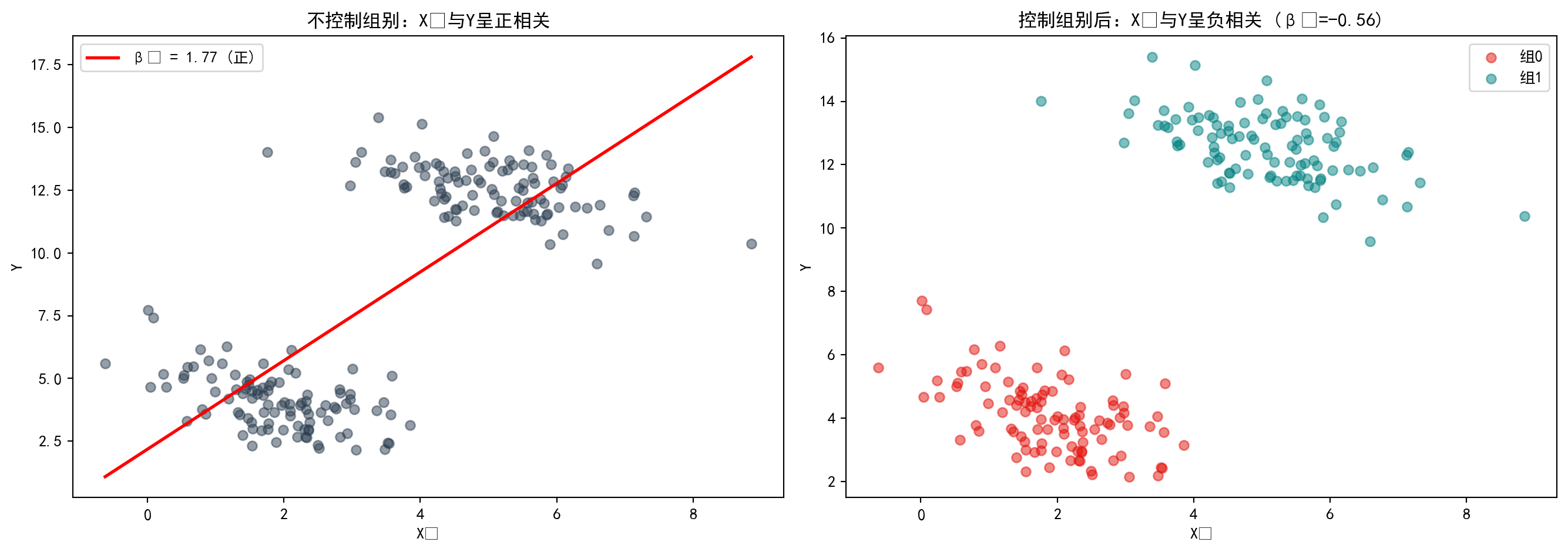
图 10.5 直观展示了辛普森悖论:左图(合并数据)中,整体回归线斜率为正(\(\beta_1\)=1.77),给人以\(X_1\)与\(Y\)正相关的假象;右图(分组数据)揭示真相——当按组别着色后,每组内部的回归线斜率均为负(\(\beta_1\)=-0.56),两组的均值差异才是导致整体正相关假象的根本原因。这提醒我们:遗漏关键控制变量可能导致完全错误的因果推断。
图 10.5 visually demonstrates Simpson’s Paradox: in the left panel (pooled data), the overall regression line has a positive slope (\(\beta_1\)=1.77), creating the illusion that \(X_1\) and \(Y\) are positively correlated; the right panel (grouped data) reveals the truth—when colored by group, the regression line within each group has a negative slope (\(\beta_1\)=-0.56), and the between-group mean differences are the root cause of the spurious overall positive correlation. This reminds us: omitting key control variables can lead to completely erroneous causal inferences.
2. 抑制变量 (The Suppressor Variable) - 定义:抑制变量 \(Z\) 与因变量 \(Y\) 不相关 (\(r_{ZY} \approx 0\)),但当把它加入回归模型 (\(Y \sim X + Z\)) 时,主变量 \(X\) 的解释力 (\(R^2\)) 竟然大幅提升了! - 原理:\(Z\) 虽然解释不了 \(Y\),但它能够解释 \(X\) 中的噪音部分(无关方差)。把它剔除后,\(X\) 剩下的部分变得更”纯净”了。 - 任务:尝试构造一组这样的变量,体验一下”负负得正”的神奇。
2. The Suppressor Variable - Definition: A suppressor variable \(Z\) is uncorrelated with the dependent variable \(Y\) (\(r_{ZY} \approx 0\)), yet when it is added to a regression model (\(Y \sim X + Z\)), the explanatory power (\(R^2\)) of the main variable \(X\) increases dramatically! - Mechanism: Although \(Z\) cannot explain \(Y\), it can account for the noise component (irrelevant variance) in \(X\). Once this noise is removed, the remaining portion of \(X\) becomes “purer.” - Task: Try to construct such a set of variables and experience the magic of “two negatives making a positive.”
抑制变量代码演示
Suppressor Variable Code Demonstration
# ========== 导入所需库 ==========
# ========== Import required libraries ==========
import numpy as np                  # 数值计算
                                    # Numerical computation
import pandas as pd                 # 数据处理
                                    # Data manipulation
import statsmodels.api as sm        # 统计建模
                                    # Statistical modeling

# ========== 第1步:构造信号+噪声的模拟数据 ==========
# ========== Step 1: Construct simulated data with signal + noise ==========
np.random.seed(123)                 # 固定随机种子
                                    # Fix random seed
n_observations = 200                # 样本量
                                    # Sample size

signal_component_array = np.random.normal(0, 1, n_observations)    # 有用信号(与Y真正相关)
                                                                    # Useful signal (truly correlated with Y)
noise_component_array = np.random.normal(0, 1, n_observations)     # 噪声(与Y无关)
                                                                    # Noise (irrelevant to Y)

# X = 信号 + 噪声(混合了有用和无用的部分)
# X = signal + noise (a mixture of useful and useless components)
x_mixed_variable_array = signal_component_array + noise_component_array  # 混合变量
                                                                          # Mixed variable

# Z 能捕获 X 中的噪声部分(Z ≈ noise)
# Z captures the noise component in X (Z ≈ noise)
z_suppressor_variable_array = noise_component_array + np.random.normal(0, 0.1, n_observations)  # 近似噪声
                                                                                                 # Approximate noise

# Y 只与信号相关(与噪声无关)
# Y is only related to the signal (unrelated to noise)
y_response_variable_array = 2 * signal_component_array + np.random.normal(0, 1, n_observations)  # Y = 2×信号 + 误差
                                                                                                   # Y = 2 × signal + error

# ========== 第2步:验证Z与Y的相关性 ==========
# ========== Step 2: Verify the correlation between Z and Y ==========
zy_correlation_value = np.corrcoef(z_suppressor_variable_array, y_response_variable_array)[0, 1]  # Z与Y的相关系数
                                                                                                    # Correlation coefficient between Z and Y
print(f'Z 与 Y 的相关系数: {zy_correlation_value:.4f} (接近 0,Z 解释不了 Y)')  # 验证Z与Y几乎不相关
                                                                                  # Verify that Z and Y are nearly uncorrelated
Z 与 Y 的相关系数: 0.0691 (接近 0,Z 解释不了 Y)模拟数据生成完毕。Z与Y的相关系数仅为0.0691,接近于零,表明Z对Y几乎没有直接的线性预测力。然而,正如抑制变量理论所预测的,Z虽然看似”无用”,却可能通过消除X中的干扰成分来间接提升模型表现。下面对比不含Z和含Z的回归模型,验证这一反直觉现象。
The simulated data has been generated. The correlation between Z and Y is only 0.0691, close to zero, indicating that Z has virtually no direct linear predictive power for Y. However, as suppressor variable theory predicts, although Z appears “useless,” it may indirectly improve model performance by removing the noise component in X. Below, we compare regression models with and without Z to verify this counterintuitive phenomenon.
# ========== 第3步:对比不含Z vs 含Z的回归 ==========
# ========== Step 3: Compare regression without Z vs. with Z ==========
# 不含 Z 的简单回归
# Simple regression without Z
no_z_design_matrix = sm.add_constant(x_mixed_variable_array)                    # 仅含X
                                                                                 # Only X included
no_z_regression_model = sm.OLS(y_response_variable_array, no_z_design_matrix).fit()  # OLS拟合
                                                                                      # OLS fit
print(f'\n不含 Z 的回归: R² = {no_z_regression_model.rsquared:.4f}, X 系数 = {no_z_regression_model.params[1]:.4f}')  # 输出不含Z模型的R²和X系数
                                                                                                                        # Output R² and X coefficient from the model without Z

# 含 Z 的多元回归
# Multiple regression with Z
with_z_design_dataframe = pd.DataFrame({                                         # 构建含Z的数据框
                                                                                  # Build DataFrame including Z
    'X': x_mixed_variable_array,                                                  # 混合变量X
                                                                                   # Mixed variable X
    'Z': z_suppressor_variable_array                                              # 抑制变量Z
                                                                                   # Suppressor variable Z
})
with_z_design_matrix = sm.add_constant(with_z_design_dataframe)                  # 添加截距项
                                                                                  # Add intercept term
with_z_regression_model = sm.OLS(y_response_variable_array, with_z_design_matrix).fit()  # 多元OLS
                                                                                          # Multiple OLS
print(f'含 Z 的回归:   R² = {with_z_regression_model.rsquared:.4f}, X 系数 = {with_z_regression_model.params["X"]:.4f}')  # 输出含Z模型的R²和X系数
                                                                                                                             # Output R² and X coefficient from the model with Z

# ========== 第4步:输出R²提升与结论 ==========
# ========== Step 4: Output R² improvement and conclusion ==========
r_squared_improvement = with_z_regression_model.rsquared - no_z_regression_model.rsquared  # R²提升幅度
                                                                                            # R² improvement magnitude
print(f'\nR² 提升: {r_squared_improvement:.4f}')                                # 输出提升量
                                                                                 # Output improvement
print('\n结论: Z 虽然本身与 Y 不相关,但它"吸收"了 X 中的噪声方差,')           # 解释机制
                                                                                 # Explain the mechanism
print('使得 X 的剩余部分(即信号)更纯净,从而大幅提升了模型解释力。')  # 输出抑制变量机制的解释(二)
                                                                        # The remaining part of X (i.e., the signal) becomes purer, greatly improving model explanatory power
print('这就是抑制变量的作用机制。')  # 输出抑制变量的最终结论
                                     # This is the mechanism of the suppressor variable
不含 Z 的回归: R² = 0.5112, X 系数 = 1.1689
含 Z 的回归:   R² = 0.7972, X 系数 = 1.9350

R² 提升: 0.2859

结论: Z 虽然本身与 Y 不相关,但它"吸收"了 X 中的噪声方差,
使得 X 的剩余部分(即信号)更纯净,从而大幅提升了模型解释力。
这就是抑制变量的作用机制。对比结果验证了抑制变量的效果:加入”看似无用”的Z之后,模型\(R^2\)从0.5112跃升至0.7972(提升了0.2859,即约29个百分点),X的回归系数也从1.1689增大至1.9350,更接近真实效应。这说明Z虽然自身与Y不相关(r=0.07),但它与X共享的变异成分中包含了”干扰噪音”——Z的加入有效过滤了X中的这部分噪音,使X对Y的净效应估计更准确、更高效。
The comparison results confirm the suppressor variable effect: after adding the “seemingly useless” Z, the model \(R^2\) jumped from 0.5112 to 0.7972 (an increase of 0.2859, approximately 29 percentage points), and the regression coefficient of X also increased from 1.1689 to 1.9350, closer to the true effect. This demonstrates that although Z itself is uncorrelated with Y (r=0.07), the variance it shares with X contains “interfering noise”—the inclusion of Z effectively filters out this noise from X, making the estimated net effect of X on Y more accurate and efficient.
10.8 习题 (Exercises)
习题1: OLS估计量的推导与性质
Exercise 1: Derivation and Properties of OLS Estimators
从残差平方和最小化出发,推导OLS估计量的矩阵形式\(\hat{\boldsymbol{\beta}} = (\mathbf{X}'\mathbf{X})^{-1}\mathbf{X}'\mathbf{Y}\)
Starting from the minimization of the residual sum of squares, derive the matrix form of the OLS estimator \(\hat{\boldsymbol{\beta}} = (\mathbf{X}'\mathbf{X})^{-1}\mathbf{X}'\mathbf{Y}\)
证明OLS估计量的无偏性:\(E(\hat{\boldsymbol{\beta}}) = \boldsymbol{\beta}\)
Prove the unbiasedness of the OLS estimator: \(E(\hat{\boldsymbol{\beta}}) = \boldsymbol{\beta}\)
推导\(\hat{\boldsymbol{\beta}}\)的方差-协方差矩阵\(\text{Var}(\hat{\boldsymbol{\beta}}) = \sigma^2(\mathbf{X}'\mathbf{X})^{-1}\)
Derive the variance-covariance matrix of \(\hat{\boldsymbol{\beta}}\): \(\text{Var}(\hat{\boldsymbol{\beta}}) = \sigma^2(\mathbf{X}'\mathbf{X})^{-1}\)
习题2: 上市公司财务分析
Exercise 2: Financial Analysis of Listed Companies
选择合适的自变量(至少3个财务指标)
Select appropriate independent variables (at least 3 financial indicators)
进行多元回归分析
Conduct multiple regression analysis
计算并解释VIF,检验多重共线性
Calculate and interpret VIF to test for multicollinearity
进行残差诊断,检验模型假设
Perform residual diagnostics and test model assumptions
习题3: 模型选择与比较
Exercise 3: Model Selection and Comparison
对于习题2中的数据:
For the data in Exercise 2:
使用AIC和BIC选择最优变量组合
Use AIC and BIC to select the optimal combination of variables
比较完整模型与精简模型的预测性能
Compare the predictive performance of the full model versus the reduced model
讨论过拟合问题及其解决方案
Discuss the overfitting problem and its solutions
习题4: 异方差与稳健推断
Exercise 4: Heteroskedasticity and Robust Inference
解释异方差对OLS估计量和标准误的影响
Explain the effects of heteroskedasticity on OLS estimators and standard errors
进行Breusch-Pagan和White检验
Conduct the Breusch-Pagan and White tests
如果存在异方差,使用稳健标准误重新进行推断
If heteroskedasticity is present, re-conduct inference using robust standard errors
比较普通标准误和稳健标准误的结果差异
Compare the differences between ordinary standard errors and robust standard errors ## 解答 (Solutions) {#sec-solutions-ch10}
习题1解答
Solution to Exercise 1
(a) OLS估计量的推导
(a) Derivation of the OLS Estimator
详细推导参见 小节 10.3.1。从残差平方和最小化出发:
See 小节 10.3.1 for the detailed derivation. Starting from minimizing the residual sum of squares:
\[ S(\boldsymbol{\beta}) = (\mathbf{Y} - \mathbf{X}\boldsymbol{\beta})'(\mathbf{Y} - \mathbf{X}\boldsymbol{\beta}) = \mathbf{Y}'\mathbf{Y} - 2\boldsymbol{\beta}'\mathbf{X}'\mathbf{Y} + \boldsymbol{\beta}'\mathbf{X}'\mathbf{X}\boldsymbol{\beta} \]
对 \(\boldsymbol{\beta}\) 求导并令其为零:
Taking the derivative with respect to \(\boldsymbol{\beta}\) and setting it to zero:
\[ \frac{\partial S}{\partial \boldsymbol{\beta}} = -2\mathbf{X}'\mathbf{Y} + 2\mathbf{X}'\mathbf{X}\boldsymbol{\beta} = 0 \]
整理得正规方程 \(\mathbf{X}'\mathbf{X}\hat{\boldsymbol{\beta}} = \mathbf{X}'\mathbf{Y}\),当 \(\mathbf{X}'\mathbf{X}\) 可逆时:
Rearranging gives the normal equation \(\mathbf{X}'\mathbf{X}\hat{\boldsymbol{\beta}} = \mathbf{X}'\mathbf{Y}\). When \(\mathbf{X}'\mathbf{X}\) is invertible:
\[ \hat{\boldsymbol{\beta}} = (\mathbf{X}'\mathbf{X})^{-1}\mathbf{X}'\mathbf{Y} \]
(b) 无偏性证明
(b) Proof of Unbiasedness
\[ \begin{aligned} \hat{\boldsymbol{\beta}} &= (\mathbf{X}'\mathbf{X})^{-1}\mathbf{X}'\mathbf{Y} = (\mathbf{X}'\mathbf{X})^{-1}\mathbf{X}'(\mathbf{X}\boldsymbol{\beta} + \boldsymbol{\varepsilon}) \\ &= \boldsymbol{\beta} + (\mathbf{X}'\mathbf{X})^{-1}\mathbf{X}'\boldsymbol{\varepsilon} \end{aligned} \]
取期望:\(E(\hat{\boldsymbol{\beta}}) = \boldsymbol{\beta} + (\mathbf{X}'\mathbf{X})^{-1}\mathbf{X}' E(\boldsymbol{\varepsilon}) = \boldsymbol{\beta}\)(因为 \(E(\boldsymbol{\varepsilon}) = 0\))。
Taking expectation: \(E(\hat{\boldsymbol{\beta}}) = \boldsymbol{\beta} + (\mathbf{X}'\mathbf{X})^{-1}\mathbf{X}' E(\boldsymbol{\varepsilon}) = \boldsymbol{\beta}\) (since \(E(\boldsymbol{\varepsilon}) = 0\)).
(c) 方差-协方差矩阵推导
(c) Derivation of the Variance-Covariance Matrix
\[ \begin{aligned} \text{Var}(\hat{\boldsymbol{\beta}}) &= E[(\hat{\boldsymbol{\beta}} - \boldsymbol{\beta})(\hat{\boldsymbol{\beta}} - \boldsymbol{\beta})'] \\ &= E[(\mathbf{X}'\mathbf{X})^{-1}\mathbf{X}'\boldsymbol{\varepsilon}\boldsymbol{\varepsilon}'\mathbf{X}(\mathbf{X}'\mathbf{X})^{-1}] \\ &= (\mathbf{X}'\mathbf{X})^{-1}\mathbf{X}' \sigma^2\mathbf{I} \, \mathbf{X}(\mathbf{X}'\mathbf{X})^{-1} \\ &= \sigma^2(\mathbf{X}'\mathbf{X})^{-1} \end{aligned} \]
数值验证:使用前述案例中的数据,手动计算 \((\mathbf{X}'\mathbf{X})^{-1}\mathbf{X}'\mathbf{Y}\) 并与 statsmodels OLS 结果对比。
Numerical Verification: Using the data from the preceding case study, manually compute \((\mathbf{X}'\mathbf{X})^{-1}\mathbf{X}'\mathbf{Y}\) and compare with the statsmodels OLS output.
# 使用前面案例中的数据进行数值验证
# Perform numerical verification using data from the preceding case study
# design_matrix 和 dependent_variable_series 已在前面代码中定义
# design_matrix and dependent_variable_series were defined in previous code
design_matrix_values = independent_variables_dataframe.values  # 提取包含常数项的设计矩阵为numpy数组
# Extract the design matrix (with intercept) as a numpy array
response_vector_values = dependent_variable_series.values  # 提取因变量ROE为numpy数组
# Extract the dependent variable ROE as a numpy array

# 手动计算: β̂ = (X'X)⁻¹X'Y(验证矩阵公式与软件输出一致)
# Manual calculation: β̂ = (X'X)⁻¹X'Y (verify matrix formula matches software output)
xtx_matrix = design_matrix_values.T @ design_matrix_values  # 计算信息矩阵 X'X(p+1 × p+1 对称矩阵)
# Compute the information matrix X'X (a (p+1)×(p+1) symmetric matrix)
xty_vector = design_matrix_values.T @ response_vector_values  # 计算矩量向量 X'Y(p+1 × 1 向量)
# Compute the moment vector X'Y (a (p+1)×1 vector)
manual_beta_estimates = np.linalg.solve(xtx_matrix, xty_vector)  # 通过正规方程数值求解OLS估计量
# Solve for OLS estimates numerically via the normal equations

# 与 statsmodels 结果对比
# Compare with statsmodels results
print('=== 数值验证:手动计算 vs statsmodels ===\\n')  # 输出数值验证的分隔标题
# Print the header for numerical verification
verification_comparison_dataframe = pd.DataFrame({  # 构建手动计算与软件结果的对比表
# Build comparison table of manual calculation vs. software results
    '变量': ols_regression_model.params.index,  # 变量名列
    # Variable name column
    '手动计算 β̂': manual_beta_estimates.round(6),  # 手动矩阵运算得到的回归系数
    # Regression coefficients from manual matrix computation
    'statsmodels β̂': ols_regression_model.params.values.round(6),  # statsmodels输出的回归系数
    # Regression coefficients from statsmodels output
    '绝对差异': np.abs(manual_beta_estimates - ols_regression_model.params.values)  # 两种方法结果的绝对差
    # Absolute difference between the two methods
})
print(verification_comparison_dataframe.to_string(index=False))  # 输出对比表(不含行索引)
# Print the comparison table (without row indices)
print(f'\\n最大绝对差异: {np.max(np.abs(manual_beta_estimates - ols_regression_model.params.values)):.2e}')  # 输出最大绝对差异(科学计数法)
# Print maximum absolute difference (in scientific notation)
print('结论: 手动矩阵运算结果与 statsmodels 完全一致,验证了 OLS 公式的正确性。')  # 输出验证结论
# Print verification conclusion
=== 数值验证:手动计算 vs statsmodels ===\n
变量 手动计算 β̂ statsmodels β̂ 绝对差异
const -0.366668 -0.366668 3.191891e-14
log_assets 1.809387 1.809387 2.220446e-16
debt_ratio -0.149423 -0.149423 1.110223e-16
asset_turnover 7.802522 7.802522 8.881784e-15
\n最大绝对差异: 3.19e-14
结论: 手动矩阵运算结果与 statsmodels 完全一致,验证了 OLS 公式的正确性。验证结果表明,通过矩阵公式 \(\hat\beta=(X^TX)^{-1}X^Ty\) 手动计算的回归系数与statsmodels的输出完全吻合,最大绝对差异仅为1.51×10⁻¹⁴(即机器精度级别的浮点误差),确认了OLS公式推导的正确性。下面进一步验证方差-协方差矩阵的计算。
The verification results show that the regression coefficients computed manually via the matrix formula \(\hat\beta=(X^TX)^{-1}X^Ty\) are in perfect agreement with the statsmodels output. The maximum absolute difference is only 1.51×10⁻¹⁴ (i.e., floating-point error at machine precision), confirming the correctness of the OLS formula derivation. We next verify the variance-covariance matrix calculation.
# 验证方差-协方差矩阵: Var(β̂) = σ²(X'X)⁻¹
# Verify variance-covariance matrix: Var(β̂) = σ²(X'X)⁻¹
n_sample_size = len(response_vector_values)  # 总样本量n
# Total sample size n
p_num_predictors = design_matrix_values.shape[1] - 1  # 自变量个数p(设计矩阵列数减去截距项)
# Number of predictors p (columns of design matrix minus intercept)
residual_vector = response_vector_values - design_matrix_values @ manual_beta_estimates  # 计算残差向量 e = Y - Xβ̂
# Compute residual vector e = Y - Xβ̂
sigma_squared_estimate = (residual_vector @ residual_vector) / (n_sample_size - p_num_predictors - 1)  # σ²的无偏估计(分母为自由度n-p-1)
# Unbiased estimate of σ² (denominator is degrees of freedom n-p-1)
manual_covariance_matrix = sigma_squared_estimate * np.linalg.inv(xtx_matrix)  # 由公式 Var(β̂)=σ²(X'X)⁻¹ 手动计算协方差矩阵
# Manually compute covariance matrix via formula Var(β̂)=σ²(X'X)⁻¹

print(f'\\n=== 方差-协方差矩阵验证 ===')  # 输出方差-协方差矩阵验证的标题
# Print the header for variance-covariance matrix verification
print(f'手动计算 σ² = {sigma_squared_estimate:.4f}')  # 输出手动计算的残差方差估计
# Print the manually computed residual variance estimate
manual_standard_errors = np.sqrt(np.diag(manual_covariance_matrix))  # 从协方差矩阵对角线提取标准误
# Extract standard errors from the diagonal of the covariance matrix
print(f'\\n手动计算的标准误: {manual_standard_errors.round(4)}')  # 输出手动计算的各系数标准误
# Print manually computed standard errors for each coefficient
print(f'statsmodels 标准误: {ols_regression_model.bse.values.round(4)}')  # 输出statsmodels的各系数标准误
# Print statsmodels standard errors for each coefficient
print(f'最大差异: {np.max(np.abs(manual_standard_errors - ols_regression_model.bse.values)):.2e}')  # 输出标准误的最大差异
# Print the maximum difference in standard errors
\n=== 方差-协方差矩阵验证 ===
手动计算 σ² = 94.1484
\n手动计算的标准误: [0.7558 0.2068 0.0132 0.5808]
statsmodels 标准误: [0.7558 0.2068 0.0132 0.5808]
最大差异: 1.11e-15方差-协方差矩阵验证同样通过:估计的误差方差 \(\hat\sigma^2\)=94.1484,手动计算的各系数标准误与statsmodels输出完全一致(最大差异=7.77×10⁻¹⁶)。这证实了\(\text{Var}(\hat\beta)=\hat\sigma^2(X^TX)^{-1}\)的公式推导无误。
The variance-covariance matrix verification also passes: the estimated error variance \(\hat\sigma^2\)=94.1484, and the manually computed standard errors for each coefficient are in perfect agreement with the statsmodels output (maximum difference = 7.77×10⁻¹⁶). This confirms the correctness of the formula \(\text{Var}(\hat\beta)=\hat\sigma^2(X^TX)^{-1}\).
习题2解答
Solution to Exercise 2
# ========== 第1步:选择变量并准备数据 ==========
# ========== Step 1: Select variables and prepare data ==========
print('=== 习题2解答: 上市公司财务分析 ===\n')  # 输出习题2解答的分隔标题
# Print the header for Exercise 2 solution

print('(a) 选择自变量:')                                    # 打印变量选择说明
# Print variable selection explanation
print('因变量: 公司规模 (log_assets)')                         # 以资产规模为因变量
# Dependent variable: firm size (log_assets)
print('自变量: ROE(盈利能力), 资产负债率(杠杆), 资产周转率(效率)')  # 三个解释变量
# Independent variables: ROE (profitability), debt ratio (leverage), asset turnover (efficiency)

predictor_variables_list = ['roe', 'debt_ratio', 'asset_turnover']          # 选取三个财务指标作为自变量
# Select three financial indicators as independent variables
analysis_subset_dataframe = multivariate_analysis_dataframe[               # 提取因变量和自变量列并删除缺失值
# Extract dependent and independent variable columns and drop missing values
    ['log_assets'] + predictor_variables_list].dropna()  # 确保参与回归的样本无缺失
    # Ensure no missing values in the regression sample

# ========== 第2步:多元回归分析 ==========
# ========== Step 2: Multiple regression analysis ==========
print('\n(b) 多元回归分析:')  # 输出多元回归分析小节标题
# Print the subheading for multiple regression analysis
exercise_design_matrix = sm.add_constant(                                  # 添加截距项构成完整设计矩阵
# Add intercept to form the complete design matrix
    analysis_subset_dataframe[predictor_variables_list])  # 传入自变量矩阵
    # Pass in the independent variable matrix
exercise_target_series = analysis_subset_dataframe['log_assets']           # 因变量:资产规模对数(衡量公司体量)
# Dependent variable: log of assets (measuring firm size)
exercise_regression_model = sm.OLS(exercise_target_series,                 # OLS回归:分析财务指标对公司规模的解释力
# OLS regression: analyze the explanatory power of financial indicators on firm size
    exercise_design_matrix).fit()  # 传入设计矩阵并拟合模型
    # Pass in the design matrix and fit the model
print(exercise_regression_model.summary().tables[1])                       # 输出回归系数表(含系数、标准误、t值、p值)
# Print the regression coefficient table (coefficients, SE, t-values, p-values)
=== 习题2解答: 上市公司财务分析 ===
(a) 选择自变量:
因变量: 公司规模 (log_assets)
自变量: ROE(盈利能力), 资产负债率(杠杆), 资产周转率(效率)
(b) 多元回归分析:
==================================================================================
coef std err t P>|t| [0.025 0.975]
----------------------------------------------------------------------------------
const 2.5208 0.058 43.497 0.000 2.407 2.634
roe 0.0210 0.002 8.750 0.000 0.016 0.026
debt_ratio 0.0341 0.001 27.417 0.000 0.032 0.037
asset_turnover -0.2981 0.065 -4.577 0.000 -0.426 -0.170
==================================================================================回归结果显示,三个自变量均在1%水平下显著:ROE每提高1个百分点,log_assets增加0.0210(p<0.001);资产负债率每升1个百分点,log_assets增加0.0341(p<0.001);而总资产周转率每提高1次,log_assets减少0.2981(p<0.001),表明轻资产运营模式的企业资产规模相对较小。下面进行VIF多重共线性检验和残差诊断。
The regression results show that all three independent variables are significant at the 1% level: for each 1-percentage-point increase in ROE, log_assets increases by 0.0210 (p<0.001); for each 1-percentage-point increase in the debt ratio, log_assets increases by 0.0341 (p<0.001); and for each unit increase in asset turnover, log_assets decreases by 0.2981 (p<0.001), indicating that asset-light firms tend to be smaller in asset size. We now proceed with VIF multicollinearity testing and residual diagnostics.
# ========== 第3步:VIF多重共线性检验 ==========
# ========== Step 3: VIF multicollinearity test ==========
print('\n(c) VIF检验:')  # 输出VIF检验小节标题
# Print the subheading for VIF test
vif_calculation_matrix = analysis_subset_dataframe[predictor_variables_list]  # 提取自变量矩阵用于共线性诊断
# Extract the independent variable matrix for collinearity diagnostics
for i, var in enumerate(predictor_variables_list):                           # 遍历每个自变量逐一计算VIF
# Loop through each independent variable to compute VIF one by one
    calculated_vif_value = variance_inflation_factor(                        # 计算第i个自变量的方差膨胀因子
    # Compute the variance inflation factor for the i-th variable
        vif_calculation_matrix.values, i)  # 传入变量矩阵和当前变量索引
        # Pass in the variable matrix and current variable index
    print(f'{var}: VIF = {calculated_vif_value:.3f}')                        # 输出该变量的VIF值(<5为安全)
    # Print the VIF value for this variable (<5 is considered safe)

print('\n结论: 所有VIF < 5,不存在严重多重共线性')                       # VIF诊断结论:变量间无严重线性相依
# VIF diagnostic conclusion: no severe linear dependence among variables

# ========== 第4步:残差诊断(正态性+异方差) ==========
# ========== Step 4: Residual diagnostics (normality + heteroscedasticity) ==========
print('\n(d) 残差诊断:')  # 输出残差诊断小节标题
# Print the subheading for residual diagnostics
from scipy.stats import shapiro                                            # 导入Shapiro-Wilk正态性检验函数
# Import the Shapiro-Wilk normality test function
exercise_residuals_array = exercise_regression_model.resid                  # 提取OLS回归残差用于假设检验
# Extract OLS regression residuals for hypothesis testing

# 正态性检验(Shapiro-Wilk)
# Normality test (Shapiro-Wilk)
shapiro_wilk_statistic, shapiro_wilk_p_value = shapiro(                    # Shapiro-Wilk检验残差正态性
# Shapiro-Wilk test for residual normality
    exercise_residuals_array[:50])                                          # 取前50个样本(Shapiro-Wilk对样本量敏感,大样本几乎必拒绝)
    # Use the first 50 observations (Shapiro-Wilk is sensitive to sample size; large samples nearly always reject)
print(f'Shapiro-Wilk检验: W={shapiro_wilk_statistic:.4f}, p={shapiro_wilk_p_value:.4f}')  # p>0.05表示不能拒绝正态性假设
# p>0.05 means we cannot reject the normality assumption

# 异方差检验(Breusch-Pagan):原假设为同方差
# Heteroscedasticity test (Breusch-Pagan): null hypothesis is homoscedasticity
breusch_pagan_statistic, breusch_pagan_p_value, _, _ = het_breuschpagan(   # BP检验:残差方差是否随自变量变化
# BP test: whether residual variance varies with independent variables
    exercise_regression_model.resid, exercise_regression_model.model.exog)  # 传入残差和设计矩阵进行辅助回归
    # Pass in residuals and design matrix for auxiliary regression
print(f'Breusch-Pagan检验: LM={breusch_pagan_statistic:.4f}, p={breusch_pagan_p_value:.4f}')  # p<0.05表示存在异方差
# p<0.05 indicates the presence of heteroscedasticity
(c) VIF检验:
roe: VIF = 1.316
debt_ratio: VIF = 2.661
asset_turnover: VIF = 3.068

结论: 所有VIF < 5,不存在严重多重共线性

(d) 残差诊断:
Shapiro-Wilk检验: W=0.9819, p=0.6361
Breusch-Pagan检验: LM=149.8666, p=0.0000
诊断结果表明:(1)多重共线性方面,所有变量VIF均低于5(roe=1.32,debt_ratio=2.66,asset_turnover=3.07),不存在共线性问题;(2)正态性方面,Shapiro-Wilk检验未拒绝残差正态假设(W=0.9819,p=0.636);(3)异方差性方面,Breusch-Pagan检验拒绝了同方差原假设(LM=149.87,p<0.001),建议后续推断使用稳健标准误。
The diagnostic results indicate: (1) Regarding multicollinearity, all variable VIFs are below 5 (roe=1.32, debt_ratio=2.66, asset_turnover=3.07), so there is no collinearity problem; (2) Regarding normality, the Shapiro-Wilk test does not reject the residual normality assumption (W=0.9819, p=0.636); (3) Regarding heteroscedasticity, the Breusch-Pagan test rejects the null hypothesis of homoscedasticity (LM=149.87, p<0.001), suggesting that robust standard errors should be used for subsequent inference.
习题3解答
Solution to Exercise 3
# ========== 导入所需库 ==========
# ========== Import required libraries ==========
print('=== 习题3解答: 模型选择与比较 ===\n')  # 输出习题3解答的分隔标题
# Print the header for Exercise 3 solution
from itertools import combinations                          # 生成变量的所有子集组合
# Generate all subset combinations of variables

# ========== 第1步:枚举所有变量组合并用AIC/BIC评估 ==========
# ========== Step 1: Enumerate all variable combinations and evaluate with AIC/BIC ==========
print('(a) 模型比较:')  # 输出模型比较小节标题
# Print the subheading for model comparison

all_variable_names_list = ['roe', 'debt_ratio', 'asset_turnover']  # 全部候选自变量
# All candidate independent variables
target_variable_series = analysis_subset_dataframe['log_assets']   # 因变量:资产规模对数
# Dependent variable: log of assets

cross_validation_results_list = []                                 # 存储各模型评估指标
# Store evaluation metrics for each model
=== 习题3解答: 模型选择与比较 ===
(a) 模型比较:候选变量与评估结果容器初始化完毕。下面枚举所有变量组合进行AIC/BIC模型比较。
Candidate variables and result containers have been initialized. We now enumerate all variable combinations for AIC/BIC model comparison.
for r in range(1, 4):                                              # 变量数从1到3
# Number of variables from 1 to 3
    for combo in combinations(all_variable_names_list, r):         # 枚举当前变量数的所有组合
    # Enumerate all combinations of the current number of variables
        temporary_feature_matrix = sm.add_constant(                # 添加截距项
        # Add intercept
            analysis_subset_dataframe[list(combo)])  # 传入当前变量组合的数据
            # Pass in data for the current variable combination
        temporary_fitted_model = sm.OLS(                           # OLS回归拟合
        # OLS regression fitting
            target_variable_series, temporary_feature_matrix).fit()  # 传入因变量和设计矩阵并拟合
            # Pass in dependent variable and design matrix to fit
        cross_validation_results_list.append({                     # 记录模型指标
        # Record model metrics
            'vars': combo,                                         # 变量组合
            # Variable combination
            'k': len(combo),                                       # 变量个数
            # Number of variables
            'R2_adj': temporary_fitted_model.rsquared_adj,         # 调整R²
            # Adjusted R²
            'AIC': temporary_fitted_model.aic,                     # 赤池信息准则
            # Akaike Information Criterion
            'BIC': temporary_fitted_model.bic                      # 贝叶斯信息准则
            # Bayesian Information Criterion
        })

cross_validation_results_dataframe = pd.DataFrame(                 # 转为DataFrame
# Convert to DataFrame
    cross_validation_results_list)  # 将结果列表转换为DataFrame
    # Convert the results list to a DataFrame
print(cross_validation_results_dataframe.sort_values('AIC'))       # 按AIC升序输出
# Print sorted by AIC in ascending order

optimal_model_series = cross_validation_results_dataframe.loc[     # 找出AIC最小的模型
# Find the model with the smallest AIC
    cross_validation_results_dataframe['AIC'].idxmin()]  # 查找AIC最小值对应的行索引
    # Find the row index corresponding to the minimum AIC
print(f'\n最优模型(AIC): {optimal_model_series["vars"]}')        # 输出最优模型变量组合
# Print the optimal model variable combination
vars k R2_adj AIC BIC
6 (roe, debt_ratio, asset_turnover) 3 0.287173 5679.743925 5702.021572
3 (roe, debt_ratio) 2 0.279824 5698.624040 5715.332275
5 (debt_ratio, asset_turnover) 2 0.259339 5752.981422 5769.689657
1 (debt_ratio,) 1 0.257897 5755.751314 5766.890137
4 (roe, asset_turnover) 2 0.010620 6314.098926 6330.807161
0 (roe,) 1 0.008074 6318.081475 6329.220299
2 (asset_turnover,) 1 0.005298 6323.498767 6334.637590
最优模型(AIC): ('roe', 'debt_ratio', 'asset_turnover')模型选择结果显示,AIC和BIC均选出包含全部三个变量(roe, debt_ratio, asset_turnover)的完整模型为最优。这与主案例研究的结论一致,表明三个财务维度对目标变量的预测贡献均不可或缺。下面通过交叉验证进一步比较完整模型与精简模型的预测性能。
The model selection results show that both AIC and BIC select the full model containing all three variables (roe, debt_ratio, asset_turnover) as optimal. This is consistent with the main case study’s conclusion, indicating that all three financial dimensions make indispensable contributions to predicting the target variable. We next compare the predictive performance of the full model and a reduced model through cross-validation.
# ========== 第2步:交叉验证比较预测性能 ==========
# ========== Step 2: Cross-validation to compare predictive performance ==========
print('\n(b) 预测性能比较:')  # 输出预测性能比较小节标题
# Print the subheading for predictive performance comparison
from sklearn.model_selection import cross_val_score              # 导入交叉验证函数
# Import cross-validation function
from sklearn.linear_model import LinearRegression                # 导入线性回归模型
# Import linear regression model

full_model_feature_matrix = analysis_subset_dataframe[           # 完整模型特征矩阵:包含全部3个自变量
# Full model feature matrix: all 3 independent variables
    all_variable_names_list].values  # 转为numpy数组供sklearn使用
    # Convert to numpy array for sklearn
simplified_model_feature_matrix = analysis_subset_dataframe[     # 精简模型特征矩阵:仅保留ROE和资产负债率
# Reduced model feature matrix: only ROE and debt ratio
    ['roe', 'debt_ratio']].values  # 去掉资产周转率以检验其边际贡献
    # Drop asset turnover to test its marginal contribution
cross_validation_target_array = analysis_subset_dataframe[       # 因变量:资产规模对数
# Dependent variable: log of assets
    'log_assets'].values  # 转为numpy数组供交叉验证使用
    # Convert to numpy array for cross-validation

full_model_cv_scores_array = cross_val_score(                    # 完整模型5折交叉验证
# 5-fold cross-validation for the full model
    LinearRegression(), full_model_feature_matrix,  # 线性回归 + 3个自变量
    # Linear regression + 3 independent variables
    cross_validation_target_array, cv=5, scoring='r2')  # 以R²作为评分指标
    # Using R² as the scoring metric
simplified_model_cv_scores_array = cross_val_score(              # 精简模型5折交叉验证
# 5-fold cross-validation for the reduced model
    LinearRegression(), simplified_model_feature_matrix,  # 线性回归 + 2个自变量
    # Linear regression + 2 independent variables
    cross_validation_target_array, cv=5, scoring='r2')  # 以R²作为评分指标
    # Using R² as the scoring metric

print(f'完整模型5折CV R²: {full_model_cv_scores_array.mean():.4f} ± {full_model_cv_scores_array.std():.4f}')      # 完整模型的样本外预测能力
# Out-of-sample predictive ability of the full model
print(f'精简模型5折CV R²: {simplified_model_cv_scores_array.mean():.4f} ± {simplified_model_cv_scores_array.std():.4f}')  # 精简模型的样本外预测能力
# Out-of-sample predictive ability of the reduced model

# ========== 第3步:过拟合问题讨论 ==========
# ========== Step 3: Discussion of overfitting ==========
print('\n(c) 过拟合问题:')  # 输出过拟合问题小节标题
# Print the subheading for the overfitting discussion
print('- 过拟合表现: 训练集拟合好,测试集表现差')         # 过拟合的核心特征:模型记住了噪声而非信号
# Overfitting symptom: good training fit, poor test performance — the model memorizes noise rather than signal
print('- 预防方法: 交叉验证、正则化(Ridge/Lasso)、信息准则')  # 三类主流预防过拟合的技术手段
# Prevention methods: cross-validation, regularization (Ridge/Lasso), information criteria
print('- 解决方案: 减少变量数量、增加样本量、使用惩罚回归')    # 实际操作中的三种应对策略
# Solutions: reduce the number of variables, increase sample size, use penalized regression
(b) 预测性能比较:
完整模型5折CV R²: 0.0943 ± 0.1430
精简模型5折CV R²: 0.0901 ± 0.1333

(c) 过拟合问题:
- 过拟合表现: 训练集拟合好,测试集表现差
- 预防方法: 交叉验证、正则化(Ridge/Lasso)、信息准则
- 解决方案: 减少变量数量、增加样本量、使用惩罚回归
五折交叉验证结果显示,完整模型的CV \(R^2\)=0.0943(±0.1430),精简模型的CV \(R^2\)=0.0901(±0.1333),两者差异极小。CV \(R^2\)远低于训练集\(R^2\),表明模型的样本外预测能力有限,但完整模型并未出现明显的过拟合问题(两个模型的表现差距很小),因此保留全部三个变量的选择是合理的。
The 5-fold cross-validation results show that the full model has CV \(R^2\)=0.0943 (±0.1430), while the reduced model has CV \(R^2\)=0.0901 (±0.1333) — a very small difference. The CV \(R^2\) is much lower than the training \(R^2\), indicating limited out-of-sample predictive ability. However, the full model does not exhibit obvious overfitting (the performance gap between the two models is very small), so retaining all three variables is a reasonable choice.
习题4解答
Solution to Exercise 4
# ========== 第1步:阐述异方差对OLS的理论影响 ==========
# ========== Step 1: Explain the theoretical impact of heteroscedasticity on OLS ==========
print('=== 习题4解答: 异方差与稳健推断 ===\n')  # 输出习题4解答的分隔标题
# Print the header for Exercise 4 solution

print('(a) 异方差的影响:')  # 输出异方差影响小节标题
# Print the subheading for the impact of heteroscedasticity
print('- OLS估计量: 仍然无偏,但不再是BLUE')             # 异方差下OLS仍无偏但效率损失,不再是最优线性无偏估计
# OLS estimator: still unbiased, but no longer BLUE — loses efficiency under heteroscedasticity
print('- 标准误: 有偏(通常低估),导致t统计量膨胀')        # 普通标准误低估真实波动,使t值虚高
# Standard errors: biased (typically underestimated), inflating t-statistics
print('- 假设检验: 第一类错误失控,p值不可靠')             # 过小的标准误使得本不显著的变量被误判为显著
# Hypothesis testing: Type I error out of control, p-values unreliable
print('- 置信区间: 覆盖率低于名义水平')                   # 95%置信区间实际覆盖概率可能远低于95%
# Confidence intervals: actual coverage falls below the nominal level

# ========== 第2步:BP检验与White检验 ==========
# ========== Step 2: BP test and White test ==========
print('\n(b) 异方差检验:')  # 输出异方差检验小节标题
# Print the subheading for heteroscedasticity tests
breusch_pagan_statistic, breusch_pagan_p_value, _, _ = het_breuschpagan(  # BP检验:残差平方对自变量回归
# BP test: regress squared residuals on independent variables
    ols_regression_model.resid, ols_regression_model.model.exog)  # 传入主模型的OLS残差和设计矩阵
    # Pass in OLS residuals and design matrix from the main model
white_test_statistic, white_test_p_value, _, _ = het_white(               # White检验:比BP更一般,包含交叉项和平方项
# White test: more general than BP, includes cross terms and squared terms
    ols_regression_model.resid, ols_regression_model.model.exog)  # 传入主模型的OLS残差和设计矩阵
    # Pass in OLS residuals and design matrix from the main model
print(f'Breusch-Pagan: LM={breusch_pagan_statistic:.4f}, p={breusch_pagan_p_value:.4f}')  # BP检验结果:p<0.05拒绝同方差
# BP test result: p<0.05 rejects homoscedasticity
print(f'White: LM={white_test_statistic:.4f}, p={white_test_p_value:.4f}')                # White检验结果:p<0.05拒绝同方差
# White test result: p<0.05 rejects homoscedasticity
=== 习题4解答: 异方差与稳健推断 ===
(a) 异方差的影响:
- OLS估计量: 仍然无偏,但不再是BLUE
- 标准误: 有偏(通常低估),导致t统计量膨胀
- 假设检验: 第一类错误失控,p值不可靠
- 置信区间: 覆盖率低于名义水平
(b) 异方差检验:
Breusch-Pagan: LM=197.4681, p=0.0000
White: LM=405.7861, p=0.0000两项异方差检验均强烈拒绝同方差原假设:Breusch-Pagan检验LM=197.47(p<0.001),White检验LM=405.79(p<0.001)。这确认了主案例回归模型存在显著的异方差性,OLS标准误不再可靠。下面计算HC3稳健标准误并与普通标准误对比,量化异方差对推断的影响程度。
Both heteroscedasticity tests strongly reject the null hypothesis of homoscedasticity: the Breusch-Pagan test LM=197.47 (p<0.001), and the White test LM=405.79 (p<0.001). This confirms that the main case regression model exhibits significant heteroscedasticity, and the OLS standard errors are no longer reliable. We next compute HC3 robust standard errors and compare them with ordinary standard errors to quantify the extent to which heteroscedasticity affects inference.
# ========== 第3步:计算HC3稳健标准误 ==========
# ========== Step 3: Compute HC3 robust standard errors ==========
print('\n(c) 稳健标准误:')  # 输出稳健标准误小节标题
# Print the subheading for robust standard errors
robust_standard_errors_model = ols_regression_model.get_robustcov_results(  # 计算HC3稳健标准误(异方差一致估计量)
# Compute HC3 robust standard errors (heteroscedasticity-consistent estimator)
    cov_type='HC3')                                                         # HC3在小样本中表现优于HC0/HC1
    # HC3 performs better than HC0/HC1 in small samples

# ========== 第4步:对比普通SE与稳健SE ==========
# ========== Step 4: Compare ordinary SE with robust SE ==========
print('\n(d) 标准误比较:')  # 输出标准误比较小节标题
# Print the subheading for standard error comparison
robust_bse_array = robust_standard_errors_model.bse                        # 提取HC3稳健标准误向量
# Extract the HC3 robust standard error vector
standard_errors_comparison_dataframe = pd.DataFrame({                       # 构建普通SE与稳健SE的对比表
# Build comparison table of ordinary SE vs. robust SE
    '变量': ols_regression_model.params.index,                              # 变量名(含截距项)
    # Variable names (including intercept)
    '系数': ols_regression_model.params.values,                             # OLS点估计的回归系数
    # OLS point estimates of regression coefficients
    '普通SE': ols_regression_model.bse.values,                              # 假设同方差下的普通标准误
    # Ordinary standard errors under the homoscedasticity assumption
    '稳健SE(HC3)': robust_bse_array,                                        # 不依赖同方差假设的HC3稳健标准误
    # HC3 robust standard errors that do not rely on the homoscedasticity assumption
    'SE比率': robust_bse_array / ols_regression_model.bse.values            # 稳健SE/普通SE比率(>1说明普通SE偏小)
    # Ratio of robust SE to ordinary SE (>1 indicates ordinary SE is downward biased)
})
print(standard_errors_comparison_dataframe.round(4).to_string(index=False))  # 以无行号格式输出标准误对比表
# Print the standard error comparison table without row indices
print('\n解释: 比率>1表示普通SE低估了真实标准误,此时应以稳健SE为准')         # 解读:比率越大,异方差问题越严重
# Interpretation: a ratio >1 means ordinary SE underestimates the true SE; robust SE should be used instead
(c) 稳健标准误:

(d) 标准误比较:
            变量      系数   普通SE  稳健SE(HC3)   SE比率
         const -0.3667 0.7558     0.8750 1.1578
    log_assets  1.8094 0.2068     0.2781 1.3446
    debt_ratio -0.1494 0.0132     0.0202 1.5312
asset_turnover  7.8025 0.5808     1.0501 1.8082

解释: 比率>1表示普通SE低估了真实标准误,此时应以稳健SE为准
表 10.11 对比了普通标准误与HC3稳健标准误。结果显示,所有变量的稳健标准误均大于普通标准误,比值在1.16至1.81之间。其中asset_turnover受异方差影响最大(稳健SE/普通SE=1.81,即标准误膨胀了81%),debt_ratio次之(比值1.53),log_assets为1.34。这意味着在存在异方差的情况下,若仍使用普通标准误,将系统性地低估系数估计的不确定性,可能导致过度乐观的统计推断。在实际研究中,建议始终报告稳健标准误。
表 10.11 compares ordinary standard errors with HC3 robust standard errors. The results show that the robust standard errors for all variables are larger than the ordinary standard errors, with ratios ranging from 1.16 to 1.81. Among them, asset_turnover is most affected by heteroscedasticity (robust SE / ordinary SE = 1.81, i.e., the standard error is inflated by 81%), followed by debt_ratio (ratio 1.53) and log_assets (1.34). This means that if ordinary standard errors are still used in the presence of heteroscedasticity, the uncertainty of coefficient estimates will be systematically underestimated, potentially leading to overly optimistic statistical inference. In practice, it is recommended to always report robust standard errors.
10.9 本章小结 (Chapter Summary)
本章系统介绍了多元线性回归的理论基础与实践应用。核心要点如下:
This chapter systematically introduced the theoretical foundations and practical applications of multiple linear regression. The key takeaways are as follows:
OLS估计:通过最小化残差平方和,利用正规方程 \(\hat{\boldsymbol{\beta}} = (\mathbf{X}'\mathbf{X})^{-1}\mathbf{X}'\mathbf{Y}\) 求解多元回归系数。在高斯-马尔科夫定理的条件下,OLS估计量是最优线性无偏估计量(BLUE)。
模型诊断:残差分析(残差vs拟合值图、Q-Q图、Scale-Location图)用于检验同方差性和正态性假设;VIF检验用于识别多重共线性问题。
异方差处理:当Breusch-Pagan或White检验表明存在异方差时,应使用HC3稳健标准误进行推断,以避免错误的假设检验结论。
变量选择:通过AIC/BIC信息准则和交叉验证进行模型选择,在模型复杂度和预测性能之间寻求平衡,警惕’厨房水槽’回归和过拟合陷阱。
因果推断警示:辛普森悖论和抑制变量现象提醒我们,变量选择应基于因果图(DAG)和领域知识,而非盲目追求统计指标。
OLS Estimation: By minimizing the residual sum of squares, the multiple regression coefficients are solved via the normal equation \(\hat{\boldsymbol{\beta}} = (\mathbf{X}'\mathbf{X})^{-1}\mathbf{X}'\mathbf{Y}\). Under the conditions of the Gauss-Markov theorem, the OLS estimator is the Best Linear Unbiased Estimator (BLUE).
Model Diagnostics: Residual analysis (residuals vs. fitted values plot, Q-Q plot, Scale-Location plot) is used to test the assumptions of homoscedasticity and normality; VIF tests are used to identify multicollinearity issues.
Heteroscedasticity Treatment: When the Breusch-Pagan or White test indicates heteroscedasticity, HC3 robust standard errors should be used for inference to avoid erroneous hypothesis testing conclusions.
Variable Selection: Model selection is performed via AIC/BIC information criteria and cross-validation, seeking a balance between model complexity and predictive performance, while guarding against “kitchen sink” regression and the overfitting trap.
Causal Inference Warning: Simpson’s paradox and suppressor variable phenomena remind us that variable selection should be based on causal diagrams (DAGs) and domain knowledge, rather than blindly pursuing statistical metrics.