# ========== 导入所需库 ==========
# ========== Import required libraries ==========
import pandas as pd             # 数据处理库
# Data processing library
import numpy as np              # 数值计算库
# Numerical computation library
import matplotlib.pyplot as plt # 绘图库
# Plotting library
from scipy import stats         # 统计分析库
# Statistical analysis library
import platform                 # 操作系统检测库
# Operating system detection library

# ========== 第1步:设置中文字体 ==========
# ========== Step 1: Set Chinese font ==========
plt.rcParams['font.sans-serif'] = ['SimHei']   # 设置中文字体为黑体
# Set Chinese font to SimHei (bold)
plt.rcParams['axes.unicode_minus'] = False      # 正确显示负号
# Correctly display negative signs

# ========== 第2步:加载本地股价数据 ==========
# ========== Step 2: Load local stock price data ==========
# 根据操作系统选择数据路径
# Select data path based on operating system
if platform.system() == 'Windows':  # 检测当前操作系统类型
    # Detect the current operating system type
    data_path = 'C:/qiufei/data/stock'          # Windows路径
    # Windows path
else:  # 非Windows系统(Linux/Mac)
    # Non-Windows system (Linux/Mac)
    data_path = '/home/ubuntu/r2_data_mount/qiufei/data/stock'  # Linux路径
    # Linux path

# 读取前复权股价数据
# Read forward-adjusted stock price data
stock_price_dataframe = pd.read_hdf(f'{data_path}/stock_price_pre_adjusted.h5')  # 加载本地前复权股价数据
# Load local forward-adjusted stock price data
stock_price_dataframe = stock_price_dataframe.reset_index()  # 重置索引以便按列筛选
# Reset index for column-based filtering3 概率基础 (Probability Basics)
概率论是统计学的数学基础,它为从样本推断总体提供了理论框架。在商业决策中,概率思维帮助我们在不确定性的环境下做出理性的判断和选择。本章将系统介绍概率的基本概念、计算规则及其在商业实践中的应用。
Probability theory is the mathematical foundation of statistics, providing a theoretical framework for making inferences about populations from samples. In business decision-making, probabilistic thinking helps us make rational judgments and choices under uncertainty. This chapter systematically introduces the fundamental concepts of probability, computational rules, and their applications in business practice.
3.1 概率思维在金融领域的典型应用 (Typical Applications of Probabilistic Thinking in Finance)
概率论不是抽象的数学游戏,而是金融市场风险管理和投资决策的数学基石。以下展示概率方法在中国金融市场中的核心应用。
Probability theory is not an abstract mathematical exercise, but rather the mathematical cornerstone of risk management and investment decision-making in financial markets. The following showcases core applications of probabilistic methods in China’s financial markets.
3.1.1 应用一:信用风险中的违约概率估计 (Application 1: Default Probability Estimation in Credit Risk)
商业银行和信用评级机构的核心业务之一是评估贷款客户的违约概率(Probability of Default, PD)。基于 financial_statement.h5 中的历史财务数据(如资产负债率、流动比率、利息保障倍数),结合条件概率和贝叶斯定理,可以构建违约预测模型。例如,已知某行业整体违约率为2%,而资产负债率超过80%的公司违约率高达8%——条件概率 \(P(\text{违约}|\text{高杠杆})\) 显著高于先验概率 \(P(\text{违约})\),这正是概率论在风控实务中的直接应用。
One of the core functions of commercial banks and credit rating agencies is to assess the probability of default (PD) of loan clients. Using historical financial data from financial_statement.h5 (such as debt-to-asset ratios, current ratios, and interest coverage ratios), combined with conditional probability and Bayes’ theorem, default prediction models can be constructed. For example, if the overall default rate in a given industry is 2%, while companies with debt-to-asset ratios exceeding 80% have a default rate as high as 8%—the conditional probability \(P(\text{违约}|\text{高杠杆})\) is significantly higher than the prior probability \(P(\text{违约})\)—this is a direct application of probability theory in risk management practice.
3.1.2 应用二:期权定价中的风险中性概率 (Application 2: Risk-Neutral Probability in Option Pricing)
在衍生品定价中,“风险中性概率”(Risk-Neutral Probability)是一个核心概念。Black-Scholes模型和二叉树定价模型的理论基础都是构造一个概率空间,使得在该空间下所有资产的期望收益率等于无风险利率。投资者无需知道真实世界的概率分布,只需在风险中性概率下计算期望收现值,即可为期权定价。这是条件概率和测度变换在金融工程中最优雅的应用。
In derivative pricing, “risk-neutral probability” is a core concept. The theoretical foundations of both the Black-Scholes model and the binomial tree pricing model involve constructing a probability space under which the expected return of all assets equals the risk-free rate. Investors need not know the real-world probability distribution; they only need to compute the expected present value under the risk-neutral probability to price options. This represents the most elegant application of conditional probability and measure transformation in financial engineering.
3.1.3 应用三:投资组合的联合概率与尾部风险 (Application 3: Joint Probability and Tail Risk in Portfolios)
投资组合管理中,分析师需要理解多只资产收益率的联合概率分布。单一股票下跌5%或许并不罕见,但当投资组合中所有股票同时大幅下跌时(联合极端事件),投资者将面临灾难性损失。利用 stock_price_pre_adjusted.h5 中的历史行情数据,可以计算资产间的联合分布特征,估计极端尾部事件的发生概率,为压力测试和风险预算提供量化依据。这也为后续学习的相关分析(章节 8)和多元模型(章节 10)提供概率论基础。
In portfolio management, analysts need to understand the joint probability distribution of returns across multiple assets. A single stock declining by 5% may not be uncommon, but when all stocks in a portfolio decline sharply simultaneously (a joint extreme event), investors face catastrophic losses. Using historical market data from stock_price_pre_adjusted.h5, one can compute the joint distribution characteristics among assets and estimate the probability of extreme tail events, providing a quantitative basis for stress testing and risk budgeting. This also lays the probabilistic foundation for the correlation analysis (章节 8) and multivariate models (章节 10) covered in later chapters.
3.2 概率的定义与解释 (Definitions and Interpretations of Probability)
3.2.1 三种概率解释 (Three Interpretations of Probability)
3.2.1.1 1. 古典概率 (Classical Probability)
当样本空间有限且每个基本结果等可能时,事件A的概率定义为(见 式 3.1 ):
When the sample space is finite and each elementary outcome is equally likely, the probability of event A is defined as (see 式 3.1):
\[ P(A) = \frac{\text{事件A包含的基本结果数}}{\text{样本空间中基本结果总数}} \tag{3.1}\]
适用条件:
- 样本空间有限(有限个可能结果)
- 每个基本结果等可能
Applicable Conditions:
- Finite sample space (finite number of possible outcomes)
- Each elementary outcome is equally likely
经典例子: 抛掷均匀硬币,\(P(\text{正面}) = 1/2\)
Classic Example: Tossing a fair coin, \(P(\text{heads}) = 1/2\)
3.2.1.2 2. 频率概率 (Frequentist Probability)
当试验可以在相同条件下大量重复时,事件A的概率定义为(见 式 3.2 ):
When an experiment can be repeated a large number of times under identical conditions, the probability of event A is defined as (see 式 3.2):
\[ P(A) = \lim_{n \to \infty} \frac{\text{事件A发生的次数}}{n} \tag{3.2}\]
这是大数定律的体现:随着试验次数增加,事件的相对频率会稳定地接近其真实概率。
This is a manifestation of the Law of Large Numbers: as the number of trials increases, the relative frequency of an event will steadily approach its true probability.
理解频率概率:保险定价的原理
Understanding Frequentist Probability: The Principle of Insurance Pricing
保险公司如何确定保费?假设某保险公司有10,000份汽车保险,历史数据显示每年约有150起理赔。
How does an insurance company determine premiums? Suppose an insurance company has 10,000 auto insurance policies, and historical data shows approximately 150 claims per year.
频率概率思路:
- 理赔频率 ≈ 150/10,000 = 1.5%
- 如果平均理赔金额为50,000元
- 则期望理赔成本 = 1.5% × 50,000 = 750元/人
- 保费至少应覆盖这个成本,再加上运营费用和利润
Frequentist probability reasoning:
- Claim frequency ≈ 150/10,000 = 1.5%
- If the average claim amount is 50,000 RMB
- Then the expected claim cost = 1.5% × 50,000 = 750 RMB per person
- Premiums must at least cover this cost, plus operating expenses and profit
这就是为什么保险公司需要大量客户:只有样本足够大,频率才稳定地接近真实概率。
This is why insurance companies need a large number of policyholders: only when the sample is sufficiently large does the frequency stably approach the true probability.
3.2.1.3 3. 主观概率 (Subjective Probability)
当事件不可重复时,概率反映的是个人基于可用信息对事件发生可能性的信念程度(degree of belief)。
When events are non-repeatable, probability reflects an individual’s degree of belief in the likelihood of an event occurring, based on available information.
商业应用场景:
- 新产品成功的概率
- 某候选人当选CEO的概率
- 并购交易获得监管批准的概率
Business Application Scenarios:
- The probability of a new product’s success
- The probability of a candidate being elected CEO
- The probability of a merger or acquisition receiving regulatory approval
频率概率 vs 主观概率
Frequentist Probability vs. Subjective Probability
区分这两种解释至关重要。频率概率适用于可重复事件(如硬币抛掷),而主观概率适用于一次性事件(如某次并购是否成功)。
Distinguishing between these two interpretations is crucial. Frequentist probability applies to repeatable events (such as coin tosses), while subjective probability applies to one-time events (such as whether a particular merger will succeed).
在商业中,我们经常需要处理一次性决策,此时主观概率更有用。但要注意,主观概率应当基于证据和理性分析,而非纯粹的猜测。贝叶斯更新(Bayesian updating)为修正主观概率提供了系统方法。
In business, we frequently face one-time decisions, where subjective probability is more useful. However, it is important to note that subjective probability should be grounded in evidence and rational analysis, rather than pure guesswork. Bayesian updating provides a systematic method for revising subjective probabilities.
3.3 概率的公理化定义 (Kolmogorov’s Axioms)
柯尔莫哥洛夫建立了概率的公理化体系,这不仅是数学游戏,更是为了避免像”贝特朗悖论”那样的逻辑陷阱。 设样本空间为 \(\Omega\),事件集合为 \(\mathcal{F}\),概率测度 \(P\) 必须满足:
Kolmogorov established the axiomatic system of probability, which is not merely a mathematical exercise but serves to prevent logical traps such as “Bertrand’s paradox.” Let the sample space be \(\Omega\), the event collection be \(\mathcal{F}\); the probability measure \(P\) must satisfy:
非负性 (Non-negativity): 对任意事件 \(A \in \mathcal{F}\),\(P(A) \geq 0\)。
- 直觉:概率不可能为负(就像长度、质量不能为负)。
Non-negativity: For any event \(A \in \mathcal{F}\), \(P(A) \geq 0\).
- Intuition: Probability cannot be negative (just as length and mass cannot be negative).
规范性 (Normalization): \(P(\Omega) = 1\)。
- 直觉:某种结果肯定会发生(确定性事件的概率为 1)。
Normalization: \(P(\Omega) = 1\).
- Intuition: Some outcome is certain to occur (the probability of a certain event is 1).
可列可加性 (Countable Additivity): 对于可数个互斥事件 \(A_1, A_2, ...\)(即 \(\forall i \neq j, A_i \cap A_j = \emptyset\)): \[ P\left(\bigcup_{i=1}^{\infty} A_i\right) = \sum_{i=1}^{\infty} P(A_i) \tag{3.3}\]
Countable Additivity: For countably many mutually exclusive events \(A_1, A_2, ...\) (i.e., \(\forall i \neq j, A_i \cap A_j = \emptyset\)): \[ P\left(\bigcup_{i=1}^{\infty} A_i\right) = \sum_{i=1}^{\infty} P(A_i) \]
式 3.3 保证了概率函数在无穷可列情形下的自洽性,这是现代概率论的基石。
- 直觉:整体的概率等于各互斥部分概率之和(面积的可加性)。
式 3.3 ensures the self-consistency of the probability function in the countably infinite case, which is the cornerstone of modern probability theory.
- Intuition: The probability of the whole equals the sum of the probabilities of its mutually exclusive parts (additivity of area).
基于公理的推论: 由此三条公理,我们可以推导出所有其他规则,例如 \(P(\emptyset)=0\) 和 \(P(A) \leq 1\)。 这告诉我们,概率本质上是一种测度(Measure),就像长度、面积、体积一样。
Corollaries from the Axioms: From these three axioms, we can derive all other rules, such as \(P(\emptyset)=0\) and \(P(A) \leq 1\). This tells us that probability is essentially a measure, just like length, area, and volume.
3.4 从理论到实践:苦活累活 (From Theory to Practice: The “Dirty Work”)
概率公理在数学上是完美的,但在现实世界(尤其是金融市场)中,教科书上的假设往往会失效。如果不了解这些”残酷的现实”,模型就算算得再精确,结果也是错的。
The probability axioms are mathematically perfect, but in the real world (especially in financial markets), textbook assumptions often break down. Without understanding these “harsh realities,” even the most precisely computed models will produce incorrect results.
3.4.1 1. 独立性的崩塌 (The Collapse of Independence)
很多风险模型假设资产之间的价格变动是独立的,或者相关性是恒定的。
Many risk models assume that price movements across assets are independent, or that correlations are constant.
理论: 股票A下跌不影响股票B。
现实: 平时可能互不影响,但一旦发生危机(如2008年金融危机或2015年股灾),所有相关性都会趋向于1。大家都在卖,泥沙俱下。
后果: 分散投资(Diversification)在最需要它的时候失效了。
Theory: Stock A’s decline does not affect Stock B.
Reality: Under normal conditions they may be unrelated, but once a crisis hits (such as the 2008 financial crisis or the 2015 Chinese stock market crash), all correlations tend toward 1. Everyone is selling, and everything falls together.
Consequence: Diversification fails precisely when it is needed most.
3.4.2 2. 肥尾效应 (Fat Tails)
经典统计学喜欢假设数据服从正态分布(钟形曲线)。在正态分布下,极端事件(如6个标准差的波动)几乎不可能发生(几百万年一次)。
Classical statistics favors the assumption that data follows a normal distribution (bell curve). Under the normal distribution, extreme events (such as a 6-standard-deviation fluctuation) are virtually impossible (once in several million years).
但在金融市场中,“几百万年一次”的暴跌每隔十年就发生一次。这就是肥尾效应——极端事件发生的概率远高于正态分布的预测。
Yet in financial markets, “once-in-several-million-years” crashes occur every decade or so. This is the fat tail effect—the probability of extreme events is far higher than what the normal distribution predicts.
让我们用A股数据来验证这一点。图 3.1 展示了海康威视日收益率的实际分布与标准正态分布的对比。
Let us verify this with A-share data. 图 3.1 presents the comparison between the actual distribution of Hikvision’s daily returns and the standard normal distribution.
前复权股价数据加载完毕。下面筛选海康威视日收益率数据并分析肥尾现象。
Forward-adjusted stock price data has been loaded. Next, we filter Hikvision’s daily return data and analyze the fat tail phenomenon.
# ========== 第3步:筛选海康威视数据并计算日收益率 ==========
# ========== Step 3: Filter Hikvision data and compute daily returns ==========
# 选取海康威视(002415.XSHE)作为A股蓝筹股代表(浙江杭州,长三角地区)
# Select Hikvision (002415.XSHE) as a representative A-share blue-chip stock (Hangzhou, Zhejiang, YRD region)
hikvision_price_dataframe = stock_price_dataframe[stock_price_dataframe['order_book_id'] == '002415.XSHE'].copy()  # 筛选海康威视数据并创建副本
# Filter Hikvision data and create a copy
hikvision_price_dataframe = hikvision_price_dataframe.sort_values('date')  # 按交易日期排序
# Sort by trading date
hikvision_price_dataframe['return'] = hikvision_price_dataframe['close'].pct_change().dropna()  # 计算日收益率(百分比变化)
# Compute daily returns (percentage change)
daily_returns_array = hikvision_price_dataframe['return'].dropna().values  # 提取为numpy数组
# Extract as a NumPy array

# ========== 第4步:标准化收益率并计算肥尾概率 ==========
# ========== Step 4: Standardize returns and compute fat tail probabilities ==========
# Z-score标准化:(每日收益 - 均值) / 标准差
# Z-score standardization: (daily return - mean) / standard deviation
returns_z_scores = (daily_returns_array - daily_returns_array.mean()) / daily_returns_array.std()  # 将日收益率标准化为Z-score
# Standardize daily returns into Z-scores

# 计算超过3个标准差的经验概率(实际数据)
# Compute empirical probability of exceeding 3 standard deviations (actual data)
empirical_probability_3sigma = np.sum(np.abs(returns_z_scores) > 3) / len(returns_z_scores)  # 计算超过3σ的经验频率
# Compute empirical frequency of exceeding 3σ
# 计算正态分布理论值(双侧概率)
# Compute the theoretical normal distribution value (two-tailed probability)
normal_probability_3sigma = 2 * (1 - stats.norm.cdf(3))  # 正态分布下超过3σ的理论概率(双侧)
# Theoretical probability of exceeding 3σ under the normal distribution (two-tailed)

# ========== 第5步:输出肥尾分析结果 ==========
# ========== Step 5: Output fat tail analysis results ==========
print(f"海康威视日收益率超过3个标准差的概率:")  # 输出肥尾分析标题
# Print fat tail analysis header
print(f"正态分布理论值: {normal_probability_3sigma:.6f} (约 0.27%)")  # 输出正态分布理论概率
# Print the theoretical normal distribution probability
print(f"实际历史数据值: {empirical_probability_3sigma:.6f} (约 {empirical_probability_3sigma*100:.2f}%)")  # 输出实际经验概率
# Print the actual empirical probability
print(f"倍数关系: 实际发生的频率是理论值的 {empirical_probability_3sigma/normal_probability_3sigma:.1f} 倍")  # 输出实际与理论的倍数对比
# Print the ratio of actual frequency to theoretical value
海康威视日收益率超过3个标准差的概率:
正态分布理论值: 0.002700 (约 0.27%)
实际历史数据值: 0.015312 (约 1.53%)
倍数关系: 实际发生的频率是理论值的 5.7 倍肥尾分析结果已输出。
Fat tail analysis results have been output.
运行结果解读: 上述计算结果揭示了金融市场中一个至关重要的现象——肥尾效应 (Fat Tail)。根据正态分布的理论预测,日收益率波动超过3个标准差(即”3σ事件”)的概率仅为0.27%,意味着大约每370个交易日才会出现一次。然而,海康威视的实际历史数据显示,这类极端波动的经验概率高达1.53%,是正态分布理论值的5.7倍。换言之,在真实市场中,“黑天鹅”事件的发生频率远高于基于正态分布假设的风险模型所预期的水平。这一发现对金融风险管理具有深远的警示意义:如果投资者或风控系统仅依赖正态分布来评估尾部风险(如VaR模型),将严重低估极端损失的发生概率。
Interpretation of Results: The above calculations reveal a critically important phenomenon in financial markets—the fat tail effect. According to the normal distribution’s theoretical prediction, the probability of daily return fluctuations exceeding 3 standard deviations (i.e., a “3σ event”) is only 0.27%, implying that such an event should occur roughly once every 370 trading days. However, Hikvision’s actual historical data shows that the empirical probability of such extreme fluctuations is as high as 1.53%, which is 5.7 times the theoretical value from the normal distribution. In other words, in real markets, “black swan” events occur far more frequently than what risk models based on normal distribution assumptions would predict. This finding carries profound implications for financial risk management: if investors or risk control systems rely solely on the normal distribution to assess tail risk (such as VaR models), they will severely underestimate the probability of extreme losses.
下面绘制实际收益率分布与标准正态分布的对比图。
Below we plot the comparison between the actual return distribution and the standard normal distribution.
# ========== 第6步:绘制肥尾效应对比图 ==========
# ========== Step 6: Plot the fat tail effect comparison chart ==========
plt.figure(figsize=(10, 6))  # 创建10×6英寸画布
# Create a 10×6 inch canvas

# 绘制实际收益率的频率直方图(归一化为概率密度)
# Plot the frequency histogram of actual returns (normalized to probability density)
plt.hist(returns_z_scores, bins=100, density=True, alpha=0.6, color='blue', label='实际数据')  # 绘制标准化收益率的频率直方图
# Plot the frequency histogram of standardized returns

# 绘制标准正态分布理论曲线
# Plot the standard normal distribution theoretical curve
x_axis_values = np.linspace(-6, 6, 1000)  # 生成-6到6的1000个等距点
# Generate 1000 evenly spaced points from -6 to 6
plt.plot(x_axis_values, stats.norm.pdf(x_axis_values), 'r-', lw=2, label='标准正态分布')  # 叠加标准正态分布的概率密度曲线
# Overlay the standard normal distribution probability density curve

# ========== 第7步:设置图表参数并输出 ==========
# ========== Step 7: Configure chart parameters and output ==========
plt.xlim(-6, 6)  # 设置x轴显示范围
# Set the x-axis display range
plt.title('肥尾效应验证:实际分布的尾部比正态分布更"厚"')  # 图表标题
# Chart title
plt.xlabel('标准差 (Sigma)')  # x轴标签
# X-axis label
plt.legend()      # 显示图例
# Display the legend
plt.grid(True, alpha=0.3)  # 添加半透明网格线
# Add semi-transparent gridlines
plt.show()        # 输出图表
# Output the chart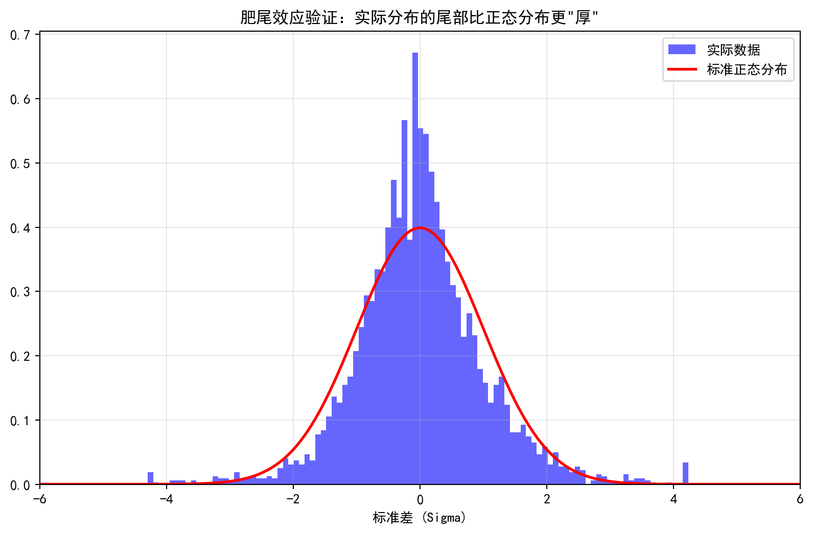
启示:永远不要盲目相信基于正态分布的风险模型(如简单的VaR)。在做压力测试时,必须考虑这些”不可能发生”的极端情况。
Takeaway: Never blindly trust risk models based on the normal distribution (such as simple VaR). When conducting stress tests, one must account for these “impossible” extreme scenarios. ## 概率的计算规则 (Rules of Probability Calculation) {#sec-probability-rules}
3.4.3 基本规则 (Basic Rules)
3.4.3.1 补事件规则 (Complement Rule)
事件A的补事件\(\bar{A}\) (A不发生)的概率由 式 3.4 给出:
The probability of the complement of event A, denoted \(\bar{A}\) (A does not occur), is given by 式 3.4:
\[ P(\bar{A}) = 1 - P(A) \tag{3.4}\]
3.4.3.2 加法规则 (Addition Rule)
对于任意两个事件A和B,加法规则如 式 3.5 所示:
For any two events A and B, the addition rule is shown in 式 3.5:
\[ P(A \cup B) = P(A) + P(B) - P(A \cap B) \tag{3.5}\]
其中 \(A \cap B\) 表示A和B同时发生。
where \(A \cap B\) denotes the simultaneous occurrence of both A and B.
特殊情况: 如果A和B互斥(mutually exclusive,即不可能同时发生),则:
Special case: If A and B are mutually exclusive (i.e., they cannot occur simultaneously), then:
\[ P(A \cup B) = P(A) + P(B) \]
理解加法规则:避免双重计数
Understanding the Addition Rule: Avoiding Double Counting
想象一个公司,30%的员工是技术背景,25%是管理背景,其中10%两者兼备。
Imagine a company where 30% of employees have a technical background, 25% have a management background, and 10% have both.
如果我们想计算”员工要么有技术背景,要么有管理背景”的概率,直接相加30% + 25% = 55%是错误的,因为这把”既是技术又是管理”的10%员工算了两次。
If we want to calculate the probability that “an employee has either a technical or a management background,” simply adding 30% + 25% = 55% is incorrect because it counts the 10% of employees who have both backgrounds twice.
正确的计算: 30% + 25% - 10% = 45%
The correct calculation: 30% + 25% - 10% = 45%
这就是为什么加法公式中要减去 \(P(A \cap B)\)。
This is why the addition formula requires subtracting \(P(A \cap B)\).
3.4.4 条件概率 (Conditional Probability)
3.4.4.1 定义 (Definition)
在事件B发生的条件下,事件A发生的条件概率为:
The conditional probability of event A occurring given that event B has occurred is:
条件概率的定义如 式 3.6 所示:
The definition of conditional probability is shown in 式 3.6:
\[ P(A|B) = \frac{P(A \cap B)}{P(B)} \tag{3.6}\]
其中 \(P(B) > 0\)。
where \(P(B) > 0\).
直观理解: \(P(A|B)\) 是在B已经发生的”缩小了的样本空间”中A发生的概率。
Intuitive understanding: \(P(A|B)\) is the probability of A occurring within the “reduced sample space” where B has already occurred.
3.4.5 独立性 (Independence)
3.4.5.1 定义 (Definition)
两个事件A和B独立,当且仅当其联合概率等于各自边际概率之积(见 式 3.7 ):
Two events A and B are independent if and only if their joint probability equals the product of their respective marginal probabilities (see 式 3.7):
\[ P(A \cap B) = P(A) \cdot P(B) \tag{3.7}\]
等价地:
Equivalently:
\[ P(A|B) = P(A) \]
或
or
\[ P(B|A) = P(B) \]
直观理解: 知道B发生与否,不影响对A发生概率的判断。
Intuitive understanding: Knowing whether B has occurred does not affect our assessment of the probability of A occurring.
独立 vs 互斥
Independence vs. Mutual Exclusivity
这是学生最容易混淆的两个概念!
These are the two concepts that students most easily confuse!
- 互斥(Mutually Exclusive): A和B不能同时发生
- 例如: “今天是周一” 和 “今天是周二” 互斥
- 独立(Independent): A发生与否不影响B的概率
- 例如: “抛硬币得正面” 和 “今天下雨” (通常)独立
- Mutually Exclusive: A and B cannot occur simultaneously
- Example: “Today is Monday” and “Today is Tuesday” are mutually exclusive
- Independent: Whether A occurs does not affect the probability of B
- Example: “A coin lands on heads” and “It rains today” are (typically) independent
关键: 如果A和B互斥且概率都为正,则它们不可能独立! 因为 \(P(A|B) = 0 \neq P(A)\)
Key point: If A and B are mutually exclusive and both have positive probabilities, then they cannot be independent! Because \(P(A|B) = 0 \neq P(A)\)
3.4.5.2 案例:股票收益率的独立性检验 (Case Study: Independence Test for Stock Returns)
什么是价格序列的自相关性?
What Is Autocorrelation in Price Series?
在金融学中,“有效市场假说”(EMH)认为股价已经充分反映了所有可用信息,因此历史价格不应该对未来价格有预测能力。如果市场是有效的,那么”今天涨”和”昨天涨”这两个事件应该是独立的——昨天的涨跌不影响今天的涨跌概率。反之,如果我们发现连续两天的涨跌方向存在显著的依赖关系(即”自相关性”),则意味着历史信息仍有预测价值,市场可能存在可被利用的”动量效应”或”反转效应”。独立性检验正是检验这一假设的核心工具。
In finance, the “Efficient Market Hypothesis” (EMH) posits that stock prices already fully reflect all available information, so historical prices should have no predictive power for future prices. If the market is efficient, then the events “today’s price goes up” and “yesterday’s price went up” should be independent — yesterday’s price movement should not affect today’s probability of a price increase. Conversely, if we find a significant dependence between two consecutive days’ price directions (i.e., “autocorrelation”), this implies that historical information still has predictive value and the market may exhibit exploitable “momentum effects” or “reversal effects.” An independence test is the core tool for testing this hypothesis.
我们利用A股连续两天的涨跌数据来检验”今天涨”与”昨天涨”是否独立。表 3.3 展示了检验结果。
We use consecutive two-day price movement data from A-shares to test whether “today’s price increase” and “yesterday’s price increase” are independent. 表 3.3 presents the test results.
# ========== 导入所需库 ==========
# ========== Import required libraries ==========
import pandas as pd   # 数据处理库
# Import the pandas library for data manipulation
import numpy as np    # 数值计算库
# Import the numpy library for numerical computation
import platform        # 操作系统检测库
# Import the platform library for OS detection

# ========== 第1步:加载本地股价数据 ==========
# ========== Step 1: Load local stock price data ==========
# 根据操作系统选择数据路径
# Select data path based on operating system
if platform.system() == 'Windows':  # 检测当前操作系统类型
    # Detect the current operating system type
    data_path = 'C:/qiufei/data/stock'          # Windows路径
    # Windows file path
else:  # 非Windows系统(Linux/Mac)
    # Non-Windows systems (Linux/Mac)
    data_path = '/home/ubuntu/r2_data_mount/qiufei/data/stock'  # Linux路径
    # Linux file path

# 读取前复权日度行情数据
# Read pre-adjusted daily stock price data
stock_price_dataframe = pd.read_hdf(f'{data_path}/stock_price_pre_adjusted.h5')  # 加载前复权日度股价数据
# Load pre-adjusted daily stock price data
stock_price_dataframe = stock_price_dataframe.reset_index()  # 重置索引
# Reset the index
前复权日度行情数据读取完毕。下面筛选海康威视2023年股价数据并标记每日涨跌方向。
Pre-adjusted daily stock price data has been loaded. Next, we filter Hikvision’s 2023 data and label the daily price direction.
# ========== 第2步:筛选海康威视2023年数据并计算涨跌 ==========
# ========== Step 2: Filter Hikvision 2023 data and calculate price movements ==========
# 海康威视(002415.XSHE):长三角安防龙头
# Hikvision (002415.XSHE): leading security company in the YRD region
hikvision_annual_price_dataframe = stock_price_dataframe[  # 筛选海康威视2023年股价数据
    # Filter Hikvision's 2023 stock price data
    (stock_price_dataframe['order_book_id'] == '002415.XSHE') &  # 股票代码
    # Stock ticker
    (stock_price_dataframe['date'] >= '2023-01-01') &            # 起始日期
    # Start date
    (stock_price_dataframe['date'] <= '2023-12-31')              # 截止日期
    # End date
].copy()  # 创建副本避免修改原数据
# Create a copy to avoid modifying the original data
hikvision_annual_price_dataframe = hikvision_annual_price_dataframe.sort_values('date')  # 按日期排序
# Sort by date

# 计算日收益率:(今日收盘价 - 昨日收盘价) / 昨日收盘价
# Calculate daily return: (Today's close - Yesterday's close) / Yesterday's close
hikvision_annual_price_dataframe['return'] = hikvision_annual_price_dataframe['close'].pct_change()  # 基于收盘价计算日百分比变化
# Calculate the daily percentage change based on closing prices
hikvision_annual_price_dataframe = hikvision_annual_price_dataframe.dropna()  # 删除首行空值
# Drop the first row with NaN values

# 将每日标记为"涨"或"跌"(收益率>0为涨)
# Label each day as "Up" or "Down" (positive return = Up)
daily_price_changes_list = ['涨' if return_value > 0 else '跌' for return_value in hikvision_annual_price_dataframe['return'].values]  # 列表推导式生成涨跌标签序列
# List comprehension to generate the sequence of up/down labels
海康威视2023年股价数据加载与涨跌分类完成。下面构建转移矩阵并检验连续日涨跌的独立性。
Hikvision’s 2023 stock price data loading and price direction classification are complete. Next, we construct the transition matrix and test the independence of consecutive daily price movements.
# ========== 第3步:构建连续两天的涨跌转移矩阵 ==========
# ========== Step 3: Construct the transition matrix for consecutive two-day price movements ==========
# 将相邻两天的涨跌状态配对,形成(第t天, 第t+1天)的元组列表
# Pair the price directions of adjacent days to form a list of (Day t, Day t+1) tuples
price_transitions_list = []  # 存储转移对
# Store transition pairs
for transition_index in range(len(daily_price_changes_list) - 1):  # 遍历每对相邻交易日
    # Iterate over each pair of adjacent trading days
    price_transitions_list.append((daily_price_changes_list[transition_index], daily_price_changes_list[transition_index+1]))  # 将(t日,t+1日)涨跌状态配对
    # Pair the price direction of day t and day t+1

transitions_dataframe = pd.DataFrame(price_transitions_list, columns=['第t天', '第t+1天'])  # 转为DataFrame
# Convert to a DataFrame

# 使用交叉表计算转移频数(含行列合计)
# Use a cross-tabulation to calculate transition frequencies (with row and column totals)
transitions_contingency_table = pd.crosstab(  # 构建涨跌转移频数交叉表
    # Construct the price direction transition contingency table
    transitions_dataframe['第t天'],      # 行:前一天状态
    # Rows: previous day's state
    transitions_dataframe['第t+1天'],    # 列:后一天状态
    # Columns: following day's state
    margins=True                          # 添加行列合计
    # Add row and column totals
)  # 完成涨跌转移交叉表的构建
# Complete the construction of the price direction transition contingency table

# ========== 第4步:输出转移频数表 ==========
# ========== Step 4: Output the transition frequency table ==========
print(f'分析股票: 海康威视(002415.XSHE)')  # 分析对象
# Print the analysis subject
print(f'分析期间: 2023年')                  # 分析时段
# Print the analysis period
print(f'交易日数: {len(hikvision_annual_price_dataframe)}')  # 样本量
# Print the number of trading days (sample size)
print('\n连续两日涨跌转移频数表:')          # 表格标题
# Table title
print(transitions_contingency_table)        # 输出交叉表
# Print the contingency table
分析股票: 海康威视(002415.XSHE)
分析期间: 2023年
交易日数: 241
连续两日涨跌转移频数表:
第t+1天 涨 跌 All
第t天
涨 41 63 104
跌 64 72 136
All 105 135 240转移频数表输出完成。下面计算条件概率并检验独立性。
The transition frequency table has been output. Next, we calculate conditional probabilities and test for independence.
# ========== 第5步:计算条件概率并检验独立性 ==========
# ========== Step 5: Calculate conditional probabilities and test for independence ==========
if '涨' in transitions_contingency_table.columns:  # 确认数据中存在"涨"列
    # Confirm that the "Up" column exists in the data
    # P(第t+1天涨 | 第t天涨) = 连续两天都涨的次数 / 第t天涨的总次数
    # P(Day t+1 Up | Day t Up) = Number of consecutive up-up days / Total number of Day t up days
    probability_up_given_up = transitions_contingency_table.loc['涨', '涨'] / transitions_contingency_table.loc['涨', 'All']  # 计算连涨的条件概率
    # Calculate the conditional probability of consecutive price increases
    # P(第t+1天涨) = 第t+1天涨的总次数 / 总转移对数(边际概率)
    # P(Day t+1 Up) = Total number of Day t+1 up / Total number of transition pairs (marginal probability)
    probability_up = transitions_contingency_table.loc['All', '涨'] / transitions_contingency_table.loc['All', 'All']  # 计算上涨的边际概率
    # Calculate the marginal probability of a price increase

    print(f'\nP(第t+1天涨 | 第t天涨) = {probability_up_given_up:.3f}')  # 条件概率
    # Conditional probability
    print(f'P(第t+1天涨) = {probability_up:.3f}')                        # 边际概率
    # Marginal probability
    # 独立性判断:若P(A|B) ≈ P(A),则事件A与B近似独立
    # Independence test: if P(A|B) ≈ P(A), then events A and B are approximately independent
    print(f'\n如果这两个概率接近,说明第t天和第t+1天的涨跌相对独立')  # 输出独立性判断结论
    # Print the independence assessment conclusion
P(第t+1天涨 | 第t天涨) = 0.394
P(第t+1天涨) = 0.438

如果这两个概率接近,说明第t天和第t+1天的涨跌相对独立
运行结果解读: 上述独立性检验的核心逻辑是比较条件概率 \(P(\text{第}t+1\text{天涨} | \text{第}t\text{天涨})\) 与边际概率 \(P(\text{第}t+1\text{天涨})\)。如果两者相等,则说明前一天的涨跌不影响后一天的走势,即日间涨跌是独立事件。计算结果显示:\(P(\text{第}t+1\text{天涨} | \text{第}t\text{天涨}) = 0.394\),略低于边际概率 \(P(\text{第}t+1\text{天涨}) = 0.438\)。两者的差异约为4.4个百分点,虽然方向上暗示海康威视2023年存在轻微的”均值回复”倾向(即涨后更容易跌),但差距并不悬殊,这与弱式有效市场假说 (Weak-Form EMH) 的预期基本一致——短期价格变动不存在强烈的可预测模式。当然,要严格判断这一差异是否具有统计显著性,需要进一步使用卡方检验等方法,这将在后续章节中介绍。
Interpretation of Results: The core logic of the independence test above is to compare the conditional probability \(P(\text{Day } t+1 \text{ Up} | \text{Day } t \text{ Up})\) with the marginal probability \(P(\text{Day } t+1 \text{ Up})\). If the two are equal, it indicates that the previous day’s price movement does not affect the next day’s trend — that is, daily price movements are independent events. The results show: \(P(\text{Day } t+1 \text{ Up} | \text{Day } t \text{ Up}) = 0.394\), slightly below the marginal probability \(P(\text{Day } t+1 \text{ Up}) = 0.438\). The difference is approximately 4.4 percentage points. Although the direction suggests a mild “mean reversion” tendency for Hikvision in 2023 (i.e., an up day is slightly more likely to be followed by a down day), the gap is not substantial. This is broadly consistent with the predictions of the Weak-Form Efficient Market Hypothesis (Weak-Form EMH) — there are no strongly predictable patterns in short-term price movements. Of course, to rigorously determine whether this difference is statistically significant, further methods such as the chi-square test are needed, which will be introduced in subsequent chapters. ## 概率计算的重要定理 (Important Theorems in Probability Calculation) {#sec-probability-theorems}
3.4.6 全概率公式 (Law of Total Probability)
设 \(B_1, B_2, ..., B_n\) 是样本空间的一个划分(partition),即它们互斥且并集为整个样本空间,则对于任意事件A,全概率公式如 式 3.8 所示:
Let \(B_1, B_2, ..., B_n\) be a partition of the sample space—that is, they are mutually exclusive and their union is the entire sample space. Then for any event A, the Law of Total Probability is given by 式 3.8:
\[ P(A) = \sum_{i=1}^{n} P(A|B_i) \cdot P(B_i) \tag{3.8}\]
直观理解: A的发生可以通过多种互斥的”途径”(\(B_i\))实现,将每种途径的概率相加即得A的总概率。
Intuitive Understanding: The occurrence of A can be realized through multiple mutually exclusive “pathways” (\(B_i\)). Summing the probability of each pathway yields the total probability of A.
全概率公式的应用:产品质量检测
Application of the Law of Total Probability: Product Quality Inspection
某公司从三家供应商采购零件:
A company procures components from three suppliers:
供应商A: 提供50%的零件,次品率2%
供应商B: 提供30%的零件,次品率3%
供应商C: 提供20%的零件,次品率5%
Supplier A: provides 50% of components, defective rate 2%
Supplier B: provides 30% of components, defective rate 3%
Supplier C: provides 20% of components, defective rate 5%
问:随机抽取一个零件,它是次品的概率?
Question: If a component is randomly selected, what is the probability that it is defective?
\[ \begin{aligned} P(\text{次品}) &= P(\text{次品}|A) \cdot P(A) \\ &\quad + P(\text{次品}|B) \cdot P(B) \\ &\quad + P(\text{次品}|C) \cdot P(C) \\ &= 0.02 \times 0.50 + 0.03 \times 0.30 + 0.05 \times 0.20 \\ &= 0.029 = 2.9\% \end{aligned} \]
3.4.7 贝叶斯定理 (Bayes’ Theorem)
贝叶斯定理描述了如何根据新证据更新我们对假设的信念。
Bayes’ Theorem describes how to update our beliefs about a hypothesis in light of new evidence.
公式(见 式 3.9 ):
Formula (see 式 3.9):
\[ P(A|B) = \frac{P(B|A) \cdot P(A)}{P(B)} \tag{3.9}\]
结合全概率公式 式 3.8 ,展开分母得到 式 3.10 :
Combining with the Law of Total Probability 式 3.8, expanding the denominator gives 式 3.10:
\[ P(A|B) = \frac{P(B|A) \cdot P(A)}{\sum_{i=1}^{n} P(B|H_i) \cdot P(H_i)} \tag{3.10}\]
其中 \(H_1, H_2, ..., H_n\) 是一个假设的划分。
where \(H_1, H_2, ..., H_n\) form a partition of hypotheses.
补充说明:贝叶斯定理的完整推导
Supplementary Note: Complete Derivation of Bayes’ Theorem
贝叶斯定理并非凭空假设,而是从条件概率的基本定义出发严格推导而来。推导过程如下:
Bayes’ Theorem is not an ad hoc assumption; it is rigorously derived from the basic definition of conditional probability. The derivation proceeds as follows:
第一步: 回顾条件概率的定义。事件 \(A\) 在事件 \(B\) 已发生条件下的概率:
Step 1: Recall the definition of conditional probability. The probability of event \(A\) given that event \(B\) has occurred:
\[ P(A|B) = \frac{P(A \cap B)}{P(B)}, \quad P(B) > 0 \]
第二步: 对称地,事件 \(B\) 在事件 \(A\) 已发生条件下的概率:
Step 2: Symmetrically, the probability of event \(B\) given that event \(A\) has occurred:
\[ P(B|A) = \frac{P(A \cap B)}{P(A)}, \quad P(A) > 0 \]
第三步: 从第二步可得联合概率的表达式:
Step 3: From Step 2, we obtain an expression for the joint probability:
\[ P(A \cap B) = P(B|A) \cdot P(A) \]
第四步: 将第三步的结果代入第一步:
Step 4: Substituting the result of Step 3 into Step 1:
\[ P(A|B) = \frac{P(B|A) \cdot P(A)}{P(B)} \]
这便是贝叶斯定理的基本形式。直觉上理解:分子 \(P(B|A) \cdot P(A)\) 衡量了”假设 \(A\) 为真时产生证据 \(B\)“的可能性大小,分母 \(P(B)\) 则起到归一化作用,确保后验概率的值在 \([0, 1]\) 范围内。
This is the basic form of Bayes’ Theorem. Intuitively, the numerator \(P(B|A) \cdot P(A)\) measures how likely it is to observe evidence \(B\) assuming hypothesis \(A\) is true, while the denominator \(P(B)\) serves as a normalizing constant, ensuring that the posterior probability lies within the \([0, 1]\) range.
第五步: 当分母 \(P(B)\) 不能直接获得时,利用全概率公式展开:
Step 5: When the denominator \(P(B)\) cannot be obtained directly, we expand it using the Law of Total Probability:
\[ P(B) = \sum_{i=1}^{n} P(B|H_i) \cdot P(H_i) \]
代入即得 式 3.10 的完整形式。全概率公式的作用是将”证据出现的总概率”分解为所有可能假设下的加权和,这在实际应用中极为常见——我们往往不知道 \(P(B)\) 的直接值,但知道在各种条件下 \(B\) 出现的概率。
Substituting yields the complete form of 式 3.10. The role of the Law of Total Probability is to decompose the “total probability of observing the evidence” into a weighted sum over all possible hypotheses—a situation that arises very frequently in practice, where we often do not know \(P(B)\) directly but do know the probability of \(B\) under each condition.
组成部分的解释:
Explanation of Components:
\(P(A)\): 先验概率(prior),在观察证据B之前对假设A的信念
\(P(B|A)\): 似然(likelihood),在假设A下观察到证据B的概率
\(P(A|B)\): 后验概率(posterior),在观察到证据B后对假设A更新的信念
\(P(A)\): Prior probability, our belief in hypothesis A before observing evidence B
\(P(B|A)\): Likelihood, the probability of observing evidence B given that hypothesis A is true
\(P(A|B)\): Posterior probability, our updated belief in hypothesis A after observing evidence B
贝叶斯定理的革命性意义
The Revolutionary Significance of Bayes’ Theorem
贝叶斯定理提供了一种学习的数学框架:
Bayes’ Theorem provides a mathematical framework for learning:
从先验知识出发 (\(P(A)\))
观察新证据 (B)
更新信念得到后验概率 (\(P(A|B)\))
Start with prior knowledge (\(P(A)\))
Observe new evidence (B)
Update beliefs to obtain the posterior probability (\(P(A|B)\))
这个过程可以迭代:今天的后验概率成为明天的先验概率,随着新证据的不断积累,我们的判断会越来越准确。
This process can be iterated: today’s posterior probability becomes tomorrow’s prior probability, and as new evidence accumulates, our judgments become increasingly accurate.
这种方法特别适合商业决策,因为商业环境充满了不确定性,我们需要不断根据新信息调整策略。这与传统的频率统计(假设参数固定)形成对比,贝叶斯方法将参数本身视为随机变量(参见 Berger 1996, American Statistician, Vol.50, No.3, pp.212-218)。
This approach is particularly well suited to business decision-making, since the business environment is rife with uncertainty and strategies must be continuously adjusted as new information arrives. This contrasts with traditional frequentist statistics (which treats parameters as fixed); the Bayesian approach treats parameters themselves as random variables (see Berger 1996, American Statistician, Vol.50, No.3, pp.212-218).
3.4.7.1 案例:上市公司财务舞弊检测的假阳性 (Case Study: False Positives in Detecting Financial Fraud among Listed Companies)
什么是假阳性问题?
What Is the False Positive Problem?
在金融监管领域,证监会和审计机构使用各种模型来识别可能存在财务造假的上市公司。这些模型的准确率通常很高,例如能正确识别99%的舞弊公司。然而,一个”反直觉”的现象是:即使模型准确率极高,当收到一次”预警”时,该公司真正存在舞弊的概率可能仍然很低。这就是著名的”假阳性悖论”(False Positive Paradox)。其根本原因在于”基础比率”(Base Rate):财务舞弊的先验概率非常低(例如仅0.1%),模型对大量正常公司产生的少量误判(假阳性)在绝对数量上远超真正的舞弊公司。贝叶斯定理正是理解和量化这一现象的核心工具,它帮助监管者在收到预警后,综合考虑先验概率来评估真实风险。
In the field of financial regulation, the CSRC (China Securities Regulatory Commission) and auditing institutions use various models to identify listed companies that may be committing financial fraud. These models typically have very high accuracy—for example, correctly identifying 99% of fraudulent companies. However, a “counter-intuitive” phenomenon arises: even when model accuracy is extremely high, the probability that a company flagged with an “alert” is actually committing fraud may still be very low. This is the well-known “False Positive Paradox.” The fundamental reason lies in the “base rate”: the prior probability of financial fraud is very low (e.g., only 0.1%), and the small number of false positives the model generates from the vast pool of normal companies far exceeds the number of truly fraudulent companies in absolute terms. Bayes’ Theorem is precisely the core tool for understanding and quantifying this phenomenon, helping regulators incorporate prior probabilities when assessing true risk after receiving an alert.
表 3.4 展示了贝叶斯定理在金融监管中的实际应用。
表 3.4 demonstrates the practical application of Bayes’ Theorem in financial regulation.
# ========== 导入所需库 ==========
# ========== Import Required Libraries ==========
import pandas as pd  # 数据处理
# Import the pandas library for data manipulation

# ========== 第1步:设定审计模型参数 ==========
# ========== Step 1: Set Audit Model Parameters ==========
# 先验概率:A股上市公司中存在财务舞弊的基础比率
# Prior probability: the base rate of financial fraud among A-share listed companies
baserate_fraud = 0.001  # 财务舞弊率(先验概率): 约0.1%
# Financial fraud rate (prior probability): approximately 0.1%
# 真阳性率(敏感度):审计模型正确识别舞弊公司的概率
# True positive rate (sensitivity): probability that the audit model correctly identifies a fraudulent company
true_positive_rate = 0.99  # 真阳性率: 99%
# True positive rate: 99%
# 假阳性率:审计模型将正常公司误判为舞弊的概率
# False positive rate: probability that the audit model incorrectly flags a normal company as fraudulent
false_positive_rate = 0.05  # 假阳性率: 5%
# False positive rate: 5%

# ========== 第2步:计算P(预警) ==========
# ========== Step 2: Calculate P(Alert) ==========
# 全概率公式:P(预警) = P(预警|舞弊)*P(舞弊) + P(预警|正常)*P(正常)
# Law of Total Probability: P(Alert) = P(Alert|Fraud)*P(Fraud) + P(Alert|Normal)*P(Normal)
probability_alert = (true_positive_rate * baserate_fraud +  # 全概率公式计算模型发出预警的总概率
              false_positive_rate * (1 - baserate_fraud))  # 模型发出预警的总概率
# Total probability that the model issues an alert, calculated via the Law of Total Probability

# ========== 第3步:计算后验概率 ==========
# ========== Step 3: Calculate the Posterior Probability ==========
# 贝叶斯定理:P(舞弊|预警) = P(预警|舞弊)*P(舞弊) / P(预警)
# Bayes' Theorem: P(Fraud|Alert) = P(Alert|Fraud)*P(Fraud) / P(Alert)
probability_fraud_given_alert = (true_positive_rate * baserate_fraud) / probability_alert  # 预警时真正舞弊的概率
# Posterior probability of actual fraud given an alert
贝叶斯条件概率计算完成。下面构建分析结果汇总表,并输出审计预警的后验概率及其实践启示。
The Bayesian conditional probability calculations are complete. Next, we construct a summary table of the analysis results and output the posterior probability of the audit alert along with its practical implications.
# ========== 第4步:构建分析结果表 ==========
# ========== Step 4: Construct the Analysis Results Table ==========
bayes_analysis_dataframe = pd.DataFrame({  # 构建贝叶斯分析结果汇总表
    # Build the Bayesian analysis summary DataFrame
    '概率类型': [  # 各概率的名称列
        # Column for probability type names
        '先验概率 P(舞弊)',      # 初始信念:上市公司舞弊的基础比率
        # Initial belief: base rate of fraud among listed companies
        '真阳性率 P(预警|舞弊)',   # 模型对真正舞弊公司的识别能力
        # Model's ability to identify truly fraudulent companies
        '假阳性率 P(预警|正常)',   # 模型对正常公司的误报率
        # Model's false alarm rate for normal companies
        '预警概率 P(预警)',       # 模型发出预警信号的总概率
        # Total probability that the model issues an alert
        '后验概率 P(舞弊|预警)'    # 收到预警后真正存在舞弊的概率
        # Probability of actual fraud given an alert has been received
    ],  # 概率类型名称列表结束
    # End of probability type name list
    '值': [  # 各概率的数值列
        # Column for numerical values
        f'{baserate_fraud:.4f} ({baserate_fraud:.1%})',              # 舞弊基础率:小数与百分比双格式输出
        # Fraud base rate: dual format output (decimal and percentage)
        f'{true_positive_rate:.4f} ({true_positive_rate:.1%})',      # 真阳性率:审计模型对舞弊的识别能力
        # True positive rate: audit model's fraud detection capability
        f'{false_positive_rate:.4f} ({false_positive_rate:.1%})',    # 假阳性率:正常公司被误判的风险大小
        # False positive rate: risk of misclassifying normal companies
        f'{probability_alert:.4f} ({probability_alert:.1%})',        # 预警总概率:全概率公式的计算结果
        # Total alert probability: result of the Law of Total Probability
        f'{probability_fraud_given_alert:.4f} ({probability_fraud_given_alert:.2%})'  # 后验概率:贝叶斯公式的核心输出
        # Posterior probability: the key output of Bayes' formula
    ],  # 概率数值列表结束
    # End of numerical value list
    '解释': [  # 各概率的含义说明列
        # Column for explanations
        'A股上市公司中财务舞弊的基础比率',           # 参数含义说明
        # Base rate of financial fraud among A-share listed companies
        '审计模型正确识别舞弊公司的概率',             # 参数含义说明
        # Probability that the audit model correctly identifies a fraudulent company
        '审计模型将正常公司误判为舞弊的概率',          # 参数含义说明
        # Probability that the audit model incorrectly flags a normal company
        '所有公司中收到审计预警的总概率',             # 结果说明
        # Total probability of receiving an audit alert across all companies
        '收到审计预警时该公司真正存在舞弊的概率'       # 关键结果说明
        # Probability that a company is actually fraudulent when an alert is received
    ]  # 解释说明列表结束
    # End of explanation list
})  # 完成贝叶斯分析结果DataFrame的构建
# Bayesian analysis results DataFrame construction complete
贝叶斯分析结果汇总表构建完毕。下面输出结果表格和实践启示。
The Bayesian analysis summary table has been constructed. The results table and practical insights are output below.
# ========== 第5步:输出结果 ==========
# ========== Step 5: Output Results ==========
print('贝叶斯分析结果:')  # 标题
# Print the title
print(bayes_analysis_dataframe)  # 打印分析表格
# Print the analysis table
print(f'\n结论: 即使审计模型发出预警,该公司真正存在舞弊的概率仅为 {probability_fraud_given_alert:.2%}')  # 核心发现
# Print the core finding
print('这是因为误报的公司数量远多于真正舞弊的公司数量(由于舞弊率很低)')  # 原因解释
# Explain the reason
print('启示:金融监管中,低基础率事件的检测面临严重的假阳性困扰')  # 实践启示
# Print the practical insight
贝叶斯分析结果:
概率类型 值 解释
0 先验概率 P(舞弊) 0.0010 (0.1%) A股上市公司中财务舞弊的基础比率
1 真阳性率 P(预警|舞弊) 0.9900 (99.0%) 审计模型正确识别舞弊公司的概率
2 假阳性率 P(预警|正常) 0.0500 (5.0%) 审计模型将正常公司误判为舞弊的概率
3 预警概率 P(预警) 0.0509 (5.1%) 所有公司中收到审计预警的总概率
4 后验概率 P(舞弊|预警) 0.0194 (1.94%) 收到审计预警时该公司真正存在舞弊的概率
结论: 即使审计模型发出预警,该公司真正存在舞弊的概率仅为 1.94%
这是因为误报的公司数量远多于真正舞弊的公司数量(由于舞弊率很低)
启示:金融监管中,低基础率事件的检测面临严重的假阳性困扰运行结果解读: 表 3.4 的计算结果堪称本章最具”反直觉”价值的实证发现。即便审计模型的检测能力极强(真阳性率高达99%),当基础率(先验概率)极低时——A股舞弊率仅0.1%——贝叶斯更新后的后验概率仍然非常低:预警公司中真正舞弊的概率仅为1.94%。换言之,在每100家收到预警的公司中,大约只有2家真正存在舞弊,其余98家都是”误报”。这个结论背后的数学逻辑是:虽然5%的假阳性率看似不高,但由于正常公司的基数(99.9%)远大于舞弊公司的基数(0.1%),假阳性产生的绝对数量远超真阳性。这就是贝叶斯定理中基础率谬误 (Base Rate Fallacy) 的经典体现,它警示我们在金融风控、医学诊断等低概率事件检测中,不能仅看模型的灵敏度,还必须充分考虑事件本身的基础发生率。
Interpretation of Results: The computational results in 表 3.4 represent arguably the most “counter-intuitive” empirical finding in this chapter. Even though the audit model has extremely strong detection capability (a true positive rate as high as 99%), when the base rate (prior probability) is extremely low—the A-share fraud rate is only 0.1%—the posterior probability after Bayesian updating remains very low: the probability that an alerted company is actually committing fraud is only 1.94%. In other words, out of every 100 companies that receive an alert, only about 2 are actually fraudulent, while the remaining 98 are “false alarms.” The mathematical logic behind this conclusion is that although a 5% false positive rate may seem modest, because the base of normal companies (99.9%) is far larger than the base of fraudulent companies (0.1%), the absolute number of false positives far exceeds that of true positives. This is a classic manifestation of the Base Rate Fallacy in Bayes’ Theorem, cautioning us that in financial risk management, medical diagnostics, and other low-probability event detection contexts, one must not look only at a model’s sensitivity but must also fully account for the base rate of the event itself.
贝叶斯定理在商业中的应用:客户流失预测
Application of Bayes’ Theorem in Business: Customer Churn Prediction
某电信公司想预测客户流失:
A telecommunications company wants to predict customer churn:
先验信息:
Prior Information:
整体流失率: \(P(\text{流失}) = 5\%\)
Overall churn rate: \(P(\text{Churn}) = 5\%\)
新证据:
New Evidence:
观察到客户投诉
历史数据显示: 流失客户中60%曾有投诉,留存客户中仅10%有投诉
即: \(P(\text{投诉}|\text{流失}) = 60\%\), \(P(\text{投诉}|\text{留存}) = 10\%\)
A customer complaint has been observed
Historical data show: 60% of churned customers had previously complained, while only 10% of retained customers had complaints
That is: \(P(\text{Complaint}|\text{Churn}) = 60\%\), \(P(\text{Complaint}|\text{Retained}) = 10\%\)
贝叶斯更新:
Bayesian Updating:
\[ \begin{aligned} P(\text{流失}|\text{投诉}) &= \frac{P(\text{投诉}|\text{流失}) \cdot P(\text{流失})}{P(\text{投诉})} \\ &= \frac{0.60 \times 0.05}{0.60 \times 0.05 + 0.10 \times 0.95} \\ &= \frac{0.03}{0.125} \\ &= 24\% \end{aligned} \]
结论: 观察到投诉后,客户流失的预测概率从5%上升到24%,公司应当采取挽留措施。
Conclusion: After observing a complaint, the predicted probability of customer churn rises from 5% to 24%, and the company should take retention measures. ## 概率树 (Probability Trees) {#sec-probability-trees}
概率树是一种可视化工具,用于系统地分解多阶段概率问题。
A probability tree is a visual tool used to systematically decompose multi-stage probability problems.
3.4.8 构建概率树的步骤 (Steps for Constructing a Probability Tree)
第一层: 列出所有可能的互斥结果(如:通过/不通过测试)
第二层: 对每个第一层结果,列出条件可能的后续结果
标注: 在每个分支上标注相应的概率
计算: 每个完整路径的概率 = 该路径上所有分支概率的乘积
First level: List all possible mutually exclusive outcomes (e.g., pass/fail a test)
Second level: For each first-level outcome, list the conditionally possible subsequent outcomes
Labeling: Annotate each branch with the corresponding probability
Calculation: The probability of each complete path = the product of all branch probabilities along that path
3.4.9 案例:多轮营销活动 (Case Study: Multi-Stage Marketing Campaign)
什么是营销漏斗?
What Is a Marketing Funnel?
在数字营销中,用户从看到广告到最终购买通常要经历多个阶段:曝光→打开→点击→购买,每一步都有一定比例的用户流失,整个过程形似一个”漏斗”(Marketing Funnel)。例如,企业向10,000名用户发送促销邮件,只有20%会打开邮件,打开邮件的用户中又只有15%会点击购买链接。这种多阶段、逐层递减的概率结构,正是概率树(Probability Tree)最擅长分析的场景。通过概率树,营销团队可以清晰地追踪每条用户路径的概率,计算最终转化率,并找出优化空间最大的环节。
In digital marketing, users typically go through multiple stages from seeing an advertisement to making a final purchase: exposure → open → click → purchase, with a certain proportion of users dropping off at each step. The entire process resembles a “funnel” (Marketing Funnel). For example, a company sends promotional emails to 10,000 users, but only 20% will open the email, and among those who open it, only 15% will click the purchase link. This multi-stage, progressively diminishing probability structure is precisely the type of scenario that probability trees are best suited to analyze. Through a probability tree, marketing teams can clearly trace the probability of each user path, calculate the final conversion rate, and identify the stages with the greatest potential for optimization.
图 3.2 展示了多轮营销活动各条路径的概率计算。
图 3.2 illustrates the probability calculations for each path in a multi-stage marketing campaign.
# ========== 导入所需库 ==========
# ========== Import required libraries ==========
import matplotlib.pyplot as plt       # 绘图库
# Import the plotting library
import matplotlib.patches as mpatches  # 图形补丁库(用于绘制图例等)
# Import the patches module (used for drawing legends, etc.)

# ========== 第1步:设置中文字体 ==========
# ========== Step 1: Set Chinese font ==========
plt.rcParams['font.sans-serif'] = ['SimHei']    # 设置中文字体为黑体
# Set the Chinese font to SimHei (bold)
plt.rcParams['axes.unicode_minus'] = False       # 正确显示负号
# Ensure the minus sign displays correctly

# ========== 第2步:创建画布并定义树状图节点位置 ==========
# ========== Step 2: Create the canvas and define tree node positions ==========
tree_figure, tree_axes = plt.subplots(figsize=(14, 8))  # 创建14×8英寸画布
# Create a 14×8 inch canvas

# 定义概率树各层节点的(x, y)坐标
# Define the (x, y) coordinates for each node in the probability tree
root_node = (0.1, 0.5)                    # 根节点:发送邮件
# Root node: send email
level1_left_node = (0.4, 0.75)            # 第1层左分支:打开邮件
# Level 1 left branch: opened email
level1_right_node = (0.4, 0.25)           # 第1层右分支:未打开
# Level 1 right branch: did not open
level2_left_top_node = (0.7, 0.85)        # 第2层左上:打开且购买
# Level 2 upper-left: opened and purchased
level2_left_bottom_node = (0.7, 0.65)     # 第2层左下:打开但未购买
# Level 2 lower-left: opened but did not purchase
level2_right_top_node = (0.7, 0.35)       # 第2层右上:未打开但购买
# Level 2 upper-right: did not open but purchased
level2_right_bottom_node = (0.7, 0.15)    # 第2层右下:未打开未购买
# Level 2 lower-right: did not open and did not purchase

# ========== 第3步:绘制第1层分支(发送邮件 → 打开/未打开) ==========
# ========== Step 3: Draw Level 1 branches (send email → opened/not opened) ==========
tree_axes.annotate('', xy=level1_left_node, xytext=root_node,  # 绘制根节点到左分支的箭头
# Draw arrow from root node to left branch
            arrowprops=dict(arrowstyle='->', lw=2, color='steelblue'))   # 绘制左分支箭头
# Draw left branch arrow
tree_axes.annotate('', xy=level1_right_node, xytext=root_node,  # 绘制根节点到右分支的箭头
# Draw arrow from root node to right branch
            arrowprops=dict(arrowstyle='->', lw=2, color='steelblue'))   # 绘制右分支箭头
# Draw right branch arrow

# ========== 第4步:绘制第2层分支(打开/未打开 → 购买/未购买) ==========
# ========== Step 4: Draw Level 2 branches (opened/not opened → purchased/not purchased) ==========
tree_axes.annotate('', xy=level2_left_top_node, xytext=level1_left_node,  # 绘制"打开"到"购买"的箭头
# Draw arrow from "opened" to "purchased"
            arrowprops=dict(arrowstyle='->', lw=1.5, color='darkgreen'))   # 打开→购买
# Opened → purchased
tree_axes.annotate('', xy=level2_left_bottom_node, xytext=level1_left_node,  # 绘制"打开"到"未购买"的箭头
# Draw arrow from "opened" to "not purchased"
            arrowprops=dict(arrowstyle='->', lw=1.5, color='darkgreen'))   # 打开→未购
# Opened → not purchased
tree_axes.annotate('', xy=level2_right_top_node, xytext=level1_right_node,  # 绘制"未打开"到"购买"的箭头
# Draw arrow from "not opened" to "purchased"
            arrowprops=dict(arrowstyle='->', lw=1.5, color='darkgreen'))   # 未打开→购买
# Not opened → purchased
tree_axes.annotate('', xy=level2_right_bottom_node, xytext=level1_right_node,  # 绘制"未打开"到"未购买"的箭头
# Draw arrow from "not opened" to "not purchased"
            arrowprops=dict(arrowstyle='->', lw=1.5, color='darkgreen'))   # 未打开→未购
# Not opened → not purchased
Text(0.4, 0.25, '')
概率树的分支箭头绘制完毕。下面为每个节点添加文本标签,标注事件名称及其对应的概率值:
The branch arrows of the probability tree are now drawn. Next, we add text labels to each node, annotating the event name and its corresponding probability value:
# ========== 第5步:添加各节点文本标签 ==========
# ========== Step 5: Add text labels to each node ==========
# 根节点:发送邮件
# Root node: send email
tree_axes.text(root_node[0], root_node[1], '发送邮件\n100%', ha='center', va='center',  # 根节点文本
# Root node text
        fontsize=12, bbox=dict(boxstyle='round', facecolor='wheat', alpha=0.5))  # 设置根节点字号和圆角框样式
# Set font size and rounded box style for root node
# 第1层节点:打开/未打开
# Level 1 nodes: opened/not opened
tree_axes.text(level1_left_node[0], level1_left_node[1], '打开邮件\n20%', ha='center', va='center',  # 左子节点文本
# Left child node text
        fontsize=11, bbox=dict(boxstyle='round', facecolor='lightblue', alpha=0.5))  # 浅蓝色标记"打开邮件"
# Light blue marking for "opened email"
tree_axes.text(level1_right_node[0], level1_right_node[1], '未打开\n80%', ha='center', va='center',  # 右子节点文本
# Right child node text
        fontsize=11, bbox=dict(boxstyle='round', facecolor='lightcoral', alpha=0.5))  # 浅红色标记"未打开"
# Light coral marking for "not opened"
# 第2层节点:购买/未购买
# Level 2 nodes: purchased/not purchased
tree_axes.text(level2_left_top_node[0], level2_left_top_node[1], '点击购买\n15%', ha='center', va='center',  # 打开→购买节点
# Opened → purchased node
        fontsize=10, bbox=dict(boxstyle='round', facecolor='lightgreen', alpha=0.5))  # 浅绿色标记"购买"
# Light green marking for "purchased"
tree_axes.text(level2_left_bottom_node[0], level2_left_bottom_node[1], '未购买\n85%', ha='center', va='center',  # 打开→未购买节点
# Opened → not purchased node
        fontsize=10, bbox=dict(boxstyle='round', facecolor='pink', alpha=0.5))  # 粉色标记"未购买"
# Pink marking for "not purchased"
tree_axes.text(level2_right_top_node[0], level2_right_top_node[1], '未购买\n0%', ha='center', va='center',  # 未打开→购买节点(概率0)
# Not opened → purchased node (probability 0)
        fontsize=10, bbox=dict(boxstyle='round', facecolor='pink', alpha=0.5))  # 粉色标记
# Pink marking
tree_axes.text(level2_right_bottom_node[0], level2_right_bottom_node[1], '未购买\n100%', ha='center', va='center',  # 未打开→未购买节点
# Not opened → not purchased node
        fontsize=10, bbox=dict(boxstyle='round', facecolor='pink', alpha=0.5))  # 粉色标记
# Pink marking
Text(0.7, 0.15, '未购买\n100%')树状图的节点和箭头绘制完成后,接下来添加各分支的概率标签和最终计算说明:
After the tree diagram’s nodes and arrows are drawn, we next add probability labels to each branch and the final calculation explanation:
# ========== 第6步:添加分支概率标签 ==========
# ========== Step 6: Add branch probability labels ==========
# 第1层分支概率
# Level 1 branch probabilities
tree_axes.text(0.25, 0.68, '20%', fontsize=10, color='steelblue')   # 打开邮件的概率
# Probability of opening the email
tree_axes.text(0.25, 0.32, '80%', fontsize=10, color='steelblue')   # 未打开的概率
# Probability of not opening the email
# 第2层分支概率
# Level 2 branch probabilities
tree_axes.text(0.55, 0.83, '15%', fontsize=9, color='darkgreen')    # 打开后购买的条件概率
# Conditional probability of purchasing after opening
tree_axes.text(0.55, 0.67, '85%', fontsize=9, color='darkgreen')    # 打开后未购买
# Not purchasing after opening
tree_axes.text(0.55, 0.33, '0%', fontsize=9, color='darkgreen')     # 未打开后购买的概率
# Probability of purchasing without opening
tree_axes.text(0.55, 0.17, '100%', fontsize=9, color='darkgreen')   # 未打开后未购买
# Not purchasing without opening

# ========== 第7步:设置图表参数并输出 ==========
# ========== Step 7: Set chart parameters and output ==========
tree_axes.set_xlim(0, 0.8)                # 设置x轴范围
# Set x-axis range
tree_axes.set_ylim(0, 1)                  # 设置y轴范围
# Set y-axis range
tree_axes.axis('off')                     # 隐藏坐标轴
# Hide axes
tree_axes.set_title('营销邮件响应概率树', fontsize=14, fontweight='bold')  # 设置标题
# Set the chart title

# 添加计算说明文本框
# Add a calculation explanation text box
calculation_text_box = '''
最终购买概率计算:
1. 打开且购买: 20% × 15% = 3%
2. 未打开则购买: 80% × 0% = 0%
3. 总购买概率: 3% + 0% = 3%

如果发送给10,000人,预期购买: 10,000 × 3% = 300人
'''  # 概率树计算过程的说明文本内容
# Descriptive text content for the probability tree calculation process
tree_axes.text(0.82, 0.5, calculation_text_box, fontsize=10, verticalalignment='center',  # 在树图右侧添加计算说明文本框
# Add the calculation explanation text box to the right of the tree diagram
        bbox=dict(boxstyle='round', facecolor='lightyellow', alpha=0.7))  # 设置浅黄色圆角框样式
# Set light yellow rounded box style

plt.tight_layout()  # 自动调整布局
# Automatically adjust layout
plt.show()          # 显示图表
# Display the chart
<Figure size 672x480 with 0 Axes>运行结果解读: 图 3.2 展示的概率树清楚地刻画了营销漏斗中的逐级转化过程。从根节点出发,10,000封营销邮件中仅有20%(2,000人)被打开;在打开邮件的2,000人中,又仅有15%(300人)最终完成购买;而未打开邮件的8,000人,购买概率为0。利用全概率公式,最终购买概率为:\(P(\text{购买}) = P(\text{打开}) \times P(\text{购买}|\text{打开}) + P(\text{未打开}) \times P(\text{购买}|\text{未打开}) = 0.20 \times 0.15 + 0.80 \times 0 = 3\%\)。概率树的优势在于它将复杂的多阶段条件概率计算可视化为直观的路径分析——沿每条路径将概率相乘,再将所有到达目标节点的路径概率相加,即得到最终结果。这种方法在营销ROI分析、产品推荐系统转化率建模等商业场景中有广泛应用。
Interpretation of Results: The probability tree shown in 图 3.2 clearly depicts the step-by-step conversion process within a marketing funnel. Starting from the root node, only 20% (2,000 people) of the 10,000 marketing emails are opened; among the 2,000 who opened the email, only 15% (300 people) ultimately complete a purchase; while the 8,000 people who did not open the email have a purchase probability of 0. Using the law of total probability, the final purchase probability is: \(P(\text{购买}) = P(\text{打开}) \times P(\text{购买}|\text{打开}) + P(\text{未打开}) \times P(\text{购买}|\text{未打开}) = 0.20 \times 0.15 + 0.80 \times 0 = 3\%\). The advantage of a probability tree lies in its ability to visualize complex multi-stage conditional probability calculations as intuitive path analysis—multiply the probabilities along each path, then sum the probabilities of all paths reaching the target node to obtain the final result. This method is widely applied in business scenarios such as marketing ROI analysis and conversion rate modeling for product recommendation systems.
3.5 启发式思考题 (Heuristic Problems)
1. 蒙提霍尔悖论 (Monty Hall Problem):直觉的陷阱 这是一个经典的”反直觉”问题。
1. The Monty Hall Problem: The Trap of Intuition This is a classic “counter-intuitive” problem.
场景:你有三扇门,只有一扇门后有奖品(车)。你选了门1。主持人打开门3,是空的。现在他给你机会换门2。
问题:换不换?
直觉:剩下两扇门,概率各50%,换不换无所谓。
现实:必须换! 换门后的胜率是 2/3,不换只有 1/3。
Scenario: There are three doors, and only one has a prize (a car) behind it. You choose Door 1. The host opens Door 3, which is empty. Now he gives you the chance to switch to Door 2.
Question: Should you switch?
Intuition: Two doors remain, each with a 50% probability—it doesn’t matter.
Reality: You must switch! The winning probability after switching is 2/3, while staying yields only 1/3.
我们可以用 Python 模拟来”打败”顽固的直觉。图 3.3 展示了随模拟次数增加,换门策略和不换门策略的胜率收敛过程:
We can use a Python simulation to “defeat” stubborn intuition. 图 3.3 shows the convergence of win rates for the switching and staying strategies as the number of simulations increases:
# ========== 导入所需库 ==========
# ========== Import required libraries ==========
import numpy as np              # 数值计算库
# Import the numerical computation library
import matplotlib.pyplot as plt  # 绘图库
# Import the plotting library

# ========== 第1步:定义蒙提霍尔游戏模拟函数 ==========
# ========== Step 1: Define the Monty Hall game simulation function ==========
def simulate_monty_hall_game(number_of_trials=1000):  # 定义模拟函数,默认模拟1000次
# Define the simulation function, default 1000 trials
    """ 模拟蒙提霍尔问题,返回换门与不换门的胜率 """  # 函数文档:说明输入参数与返回值
    # Docstring: Simulate the Monty Hall problem and return win rates for switching and staying
    total_wins_switch = 0   # 换门策略累计获胜次数
    # Cumulative wins for the switching strategy
    total_wins_stay = 0     # 不换门策略累计获胜次数
    # Cumulative wins for the staying strategy

    for _ in range(number_of_trials):  # 循环模拟number_of_trials次
    # Loop for the specified number of trials
        prize_door_index = np.random.randint(0, 3)    # 随机放置奖品在门0/1/2中的一扇
        # Randomly place the prize behind one of doors 0/1/2
        initial_choice_index = np.random.randint(0, 3) # 玩家随机初选一扇门
        # Player randomly selects an initial door

        # 主持人打开一扇既没有奖品也不是玩家选的门
        # The host opens a door that has no prize and was not chosen by the player
        available_doors_list = [door for door in [0, 1, 2] if door != prize_door_index and door != initial_choice_index]  # 筛选主持人可打开的门
        # Filter doors the host can open
        host_open_door_index = np.random.choice(available_doors_list)  # 主持人随机打开一扇符合条件的门
        # Host randomly opens one eligible door

        # 换门策略:选择剩下的那扇门(既不是初选也不是主持人打开的)
        # Switching strategy: choose the remaining door (neither the initial choice nor the host-opened one)
        switch_choice_index = [door for door in [0, 1, 2] if door != initial_choice_index and door != host_open_door_index][0]  # 取剩余唯一的门作为换门选择
        # Take the only remaining door as the switch choice

        if switch_choice_index == prize_door_index:  # 换门后是否中奖
        # Check if switching wins the prize
            total_wins_switch += 1  # 换门策略获胜,计数加1
            # Switching strategy wins, increment counter
        if initial_choice_index == prize_door_index:  # 不换门是否中奖
        # Check if staying wins the prize
            total_wins_stay += 1  # 不换门策略获胜,计数加1
            # Staying strategy wins, increment counter

    return total_wins_switch / number_of_trials, total_wins_stay / number_of_trials  # 返回两种策略的胜率
    # Return the win rates for both strategies
蒙提霍尔游戏模拟函数定义完毕。下面运行不同规模的模拟实验。
The Monty Hall game simulation function is now defined. Next, we run simulation experiments of varying sizes.
# ========== 第2步:运行不同规模的模拟实验 ==========
# ========== Step 2: Run simulation experiments of varying sizes ==========
win_rates_switch_list = []   # 存储各规模下换门胜率
# Store switching win rates at each scale
win_rates_stay_list = []     # 存储各规模下不换门胜率
# Store staying win rates at each scale
simulation_sizes_list = [10, 100, 1000, 10000]  # 模拟规模从10到10000递增
# Simulation sizes increasing from 10 to 10,000

for trial_size in simulation_sizes_list:  # 逐个规模运行模拟
# Run simulation for each scale
    current_switch_rate, current_stay_rate = simulate_monty_hall_game(trial_size)  # 执行模拟
    # Execute the simulation
    win_rates_switch_list.append(current_switch_rate)  # 记录换门胜率
    # Record the switching win rate
    win_rates_stay_list.append(current_stay_rate)      # 记录不换门胜率
    # Record the staying win rate
蒙提霍尔游戏模拟完成。下面绘制换门与不换门策略的胜率收敛图。
The Monty Hall game simulation is complete. Below, we plot the convergence of win rates for the switching and staying strategies.
# ========== 第3步:绘制胜率收敛图 ==========
# ========== Step 3: Plot the win rate convergence chart ==========
plt.rcParams['font.sans-serif'] = ['SimHei']    # 设置中文字体
# Set Chinese font
plt.rcParams['axes.unicode_minus'] = False       # 正确显示负号
# Ensure the minus sign displays correctly

convergence_figure, convergence_axes = plt.subplots(figsize=(10, 6))  # 创建画布
# Create the canvas
# 绘制换门策略胜率曲线
# Plot the switching strategy win rate curve
convergence_axes.plot(simulation_sizes_list, win_rates_switch_list, 'o-', color='#E3120B', label='换门胜率', linewidth=2)
# 绘制不换门策略胜率曲线
# Plot the staying strategy win rate curve
convergence_axes.plot(simulation_sizes_list, win_rates_stay_list, 's-', color='#2C3E50', label='不换胜率', linewidth=2)
# 添加理论值参考线
# Add theoretical value reference lines
convergence_axes.axhline(y=2/3, color='#E3120B', linestyle='--', alpha=0.5, label='换门理论值 (2/3)')   # 换门理论胜率
# Theoretical win rate for switching
convergence_axes.axhline(y=1/3, color='#2C3E50', linestyle='--', alpha=0.5, label='不换理论值 (1/3)')   # 不换理论胜率
# Theoretical win rate for staying

# ========== 第4步:设置图表参数并输出 ==========
# ========== Step 4: Set chart parameters and output ==========
convergence_axes.set_xscale('log')                # x轴使用对数刻度
# Use logarithmic scale for x-axis
convergence_axes.set_xlabel('模拟次数')              # x轴标签
# X-axis label
convergence_axes.set_ylabel('胜率')                    # y轴标签
# Y-axis label
convergence_axes.set_title('蒙提霍尔问题:换门策略的胜率收敛过程')  # 图表标题
# Chart title
convergence_axes.legend()                          # 显示图例
# Display legend
convergence_axes.grid(True, alpha=0.3)             # 显示网格
# Display grid
plt.tight_layout()  # 自动调整布局
# Automatically adjust layout
plt.show()          # 显示图表
# Display the chart

# ========== 第5步:输出模拟结果 ==========
# ========== Step 5: Output simulation results ==========
print(f"模拟10000次结果:")                                        # 输出标题
# Print title
print(f"换门胜率: {win_rates_switch_list[-1]:.4f} (理论值 0.6667)")  # 换门实际胜率 vs 理论值
# Switching actual win rate vs. theoretical value
print(f"不换胜率: {win_rates_stay_list[-1]:.4f} (理论值 0.3333)")    # 不换实际胜率 vs 理论值
# Staying actual win rate vs. theoretical value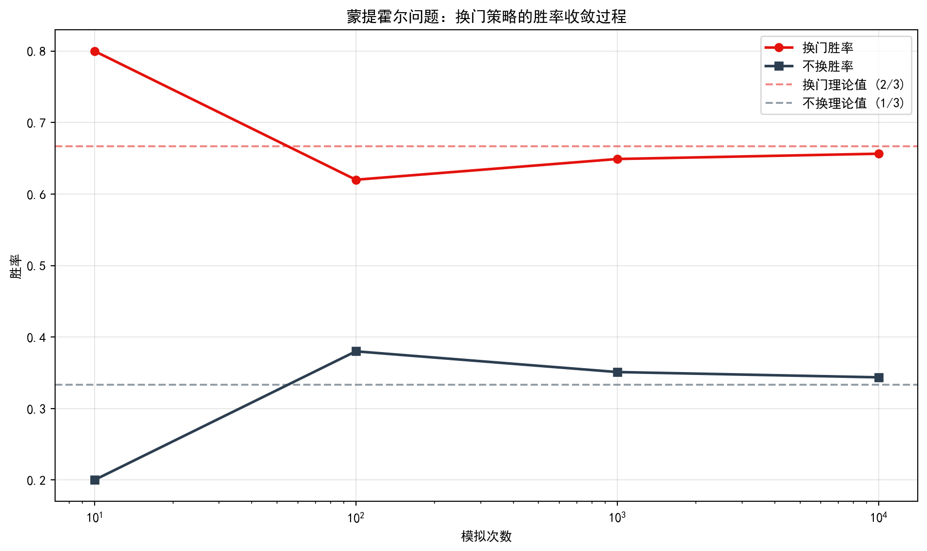
模拟10000次结果:
换门胜率: 0.6564 (理论值 0.6667)
不换胜率: 0.3436 (理论值 0.3333)原理:你初选挑中奖品的概率只有 1/3(这是不变的)。所以奖品在”剩下两扇门”里的概率是 2/3。主持人帮你排除了一扇空的,剩下的那一扇就继承了全部的 2/3 概率。
Explanation: The probability that your initial choice is correct is only 1/3 (this does not change). Therefore, the probability that the prize is behind one of the “remaining two doors” is 2/3. The host eliminates one empty door for you, so the remaining door inherits the entire 2/3 probability.
2. 生日悖论
2. The Birthday Paradox
一个房间里至少要有多少人,才能有 50% 以上的概率出现两个人同一天生日?
答案只有 23 人。
任务:尝试用概率公式 \(P(\text{至少一对}) = 1 - P(\text{全不相同})\) 进行推导。
How many people must be in a room for there to be a greater than 50% probability that two people share the same birthday?
The answer is only 23 people.
Task: Try to derive the result using the probability formula \(P(\text{至少一对}) = 1 - P(\text{全不相同})\).
3. 非传递性骰子 (Nontransitive Dice):石头剪刀布
3. Nontransitive Dice: Rock-Paper-Scissors
通常我们认为实力是传递的:如果 A > B 且 B > C,那么 A > C。
但在概率世界里,这不一定成立。
只有图灵奖得主布拉德利·埃夫隆 (Bradley Efron) 设计了4颗骰子:
- A: 4, 4, 4, 4, 0, 0
- B: 3, 3, 3, 3, 3, 3
- C: 6, 6, 2, 2, 2, 2
- D: 5, 5, 5, 1, 1, 1
神奇的性质:
- A 赢 B 的概率是 2/3
- B 赢 C 的概率是 2/3
- C 赢 D 的概率是 2/3
- 但是… D 赢 A 的概率也是 2/3!
这就像石头剪刀布一样循环相克。在商业竞争中,这意味着可能不存在”最优策略”,一切取决于你的对手是谁。
We usually assume that strength is transitive: if A > B and B > C, then A > C.
But in the world of probability, this does not necessarily hold.
Turing Award laureate Bradley Efron designed four dice:
- A: 4, 4, 4, 4, 0, 0
- B: 3, 3, 3, 3, 3, 3
- C: 6, 6, 2, 2, 2, 2
- D: 5, 5, 5, 1, 1, 1
The remarkable property:
- The probability that A beats B is 2/3
- The probability that B beats C is 2/3
- The probability that C beats D is 2/3
- However… the probability that D beats A is also 2/3!
This creates a cyclical dominance just like Rock-Paper-Scissors. In business competition, this implies that there may be no single “optimal strategy”—everything depends on who your opponent is.
4. 伯克森悖论 (Berkson’s Paradox):为什么”好男人”都有主了?
4. Berkson’s Paradox: Why Are All the “Good Men” Taken?
你是否觉得:长得帅的男生通常人品不好,通过人品好的男生通常长得不帅?
这可能不是因为上帝公平(给了一扇门关了一扇窗),而是选择偏差 (Selection Bias)。
假设相貌和人品在人群中是独立的。
但是,你只会注意到那些”要么帅,要么人品好”的人(作为潜在伴侣)。
如果一个人不帅也不好,你根本不会关注他(数据缺失)。
在这个被筛选过的样本中,相貌和人品就会表现出负相关。
商业启示:如果你只分析现有的成功客户,你可能会发现”价格敏感度”和”忠诚度”负相关,但这可能只是因为你流失了那些”既不敏感也不忠诚”的低价值客户。
Have you ever felt that good-looking men tend to have poor character, while men with good character tend not to be good-looking?
This may not be because God is fair (closing a window when opening a door), but rather due to selection bias.
Assume that appearance and character are independent in the general population.
However, you only notice people who are “either good-looking or have good character” (as potential partners).
If someone is neither good-looking nor of good character, you simply do not notice them (missing data).
In this filtered sample, appearance and character will exhibit a negative correlation.
Business insight: If you only analyze your existing successful customers, you may find that “price sensitivity” and “loyalty” are negatively correlated, but this may simply be because you have lost those “neither price-sensitive nor loyal” low-value customers. ## 思考与练习 {#sec-exercises-ch3}
3.6 Exercises
- 概率基本概念
- 从沪深300指数成分股(共300只)中随机选取一只,已知其中金融行业50只、长三角地区上市公司75只、既是金融行业又在长三角的15只,求以下概率:
- 选到金融行业股票
- 选到长三角地区上市公司
- 选到长三角金融行业股票
- 选到金融行业或长三角地区的股票
- 从沪深300指数成分股(共300只)中随机选取一只,已知其中金融行业50只、长三角地区上市公司75只、既是金融行业又在长三角的15只,求以下概率:
- Basic Probability Concepts
- A stock is randomly selected from the CSI 300 Index constituents (300 stocks in total). It is known that 50 are in the financial sector, 75 are listed companies in the Yangtze River Delta (YRD) region, and 15 are both financial sector stocks and located in the YRD. Calculate the following probabilities:
- Selecting a financial sector stock
- Selecting a YRD-region listed company
- Selecting a financial sector stock in the YRD
- Selecting a financial sector or YRD-region stock
- A stock is randomly selected from the CSI 300 Index constituents (300 stocks in total). It is known that 50 are in the financial sector, 75 are listed companies in the Yangtze River Delta (YRD) region, and 15 are both financial sector stocks and located in the YRD. Calculate the following probabilities:
- 条件概率应用
- 某公司员工数据:
- 男性占60%,女性占40%
- 男性中30%是管理者,女性中20%是管理者
- 随机选择一名员工:
- 是管理者的概率?
- 是女性管理者的概率?
- 如果是管理者,是女性的概率?
- 某公司员工数据:
- Application of Conditional Probability
- Employee data for a company:
- Males account for 60%, females account for 40%
- 30% of males are managers, 20% of females are managers
- If an employee is randomly selected:
- What is the probability of being a manager?
- What is the probability of being a female manager?
- If the employee is a manager, what is the probability of being female?
- Employee data for a company:
- 独立性检验
- 调查1000名消费者:
- 600人知道品牌A,其中300人购买
- 400人不知道品牌A,其中100人购买
- 计算:
- 知道品牌A的人的购买率
- 不知道品牌A的人的购买率
- 品牌认知和购买行为是否独立?
- 调查1000名消费者:
- Independence Test
- A survey of 1,000 consumers:
- 600 are aware of Brand A, of whom 300 made a purchase
- 400 are not aware of Brand A, of whom 100 made a purchase
- Calculate:
- The purchase rate among those aware of Brand A
- The purchase rate among those not aware of Brand A
- Are brand awareness and purchasing behavior independent?
- A survey of 1,000 consumers:
- 贝叶斯定理应用
- 某银行信贷风控模型:
- 贷款违约率: 0.5%
- 真阳性率(正确识别违约客户): 98%
- 假阳性率(误判优质客户为违约): 3%
- 如果模型预警某客户违约,该客户真正违约的概率是多少?
- 如果假阳性率降到1%,结果如何变化?
- 某银行信贷风控模型:
- Application of Bayes’ Theorem
- A bank’s credit risk control model:
- Loan default rate: 0.5%
- True positive rate (correctly identifying defaulting customers): 98%
- False positive rate (misclassifying good customers as defaulting): 3%
- If the model flags a customer as defaulting, what is the probability that the customer actually defaults?
- How does the result change if the false positive rate falls to 1%?
- A bank’s credit risk control model:
- 商业决策项目
- 选择一家上市公司,收集其过去5年的季报数据
- 计算:盈利季度后股价上涨的概率
- 使用贝叶斯方法,结合宏观经济数据(如GDP增长率),更新对下季度盈利的预测
- 撰写分析报告:如何利用概率思维进行投资决策
- Business Decision-Making Project
- Select a listed company and collect its quarterly report data over the past 5 years
- Calculate: the probability of a stock price increase following a profitable quarter
- Use Bayesian methods, combined with macroeconomic data (e.g., GDP growth rate), to update the forecast for next quarter’s earnings
- Write an analytical report: how to apply probabilistic thinking to investment decisions
3.6.1 参考答案
3.6.2 Reference Answers
习题 3.1 解答
Solution to Exercise 3.1
# ========== 导入所需库 ==========
# ========== Import Required Libraries ==========
# 本题无需额外库,仅使用基本运算
# No additional libraries needed; only basic arithmetic is used

# ========== 第1步:设定股票池参数 ==========
# ========== Step 1: Set Stock Pool Parameters ==========
print('=' * 60)  # 输出分隔线
# Print separator line
print('习题3.1解答:沪深300成分股选股概率计算')  # 输出题目标题
# Print exercise title
print('=' * 60)  # 输出分隔线
# Print separator line

# 沪深300指数成分股总数
# Total number of CSI 300 Index constituent stocks
total_stocks = 300  # 样本空间大小:沪深300成分股
# Sample space size: CSI 300 constituents
# 金融行业成分股数量(银行、证券、保险等)
# Number of financial sector constituents (banks, securities, insurance, etc.)
count_financial = 50  # 事件A:金融行业股票数量
# Event A: number of financial sector stocks
# 长三角地区(上海、江苏、浙江、安徽)上市公司数量
# Number of listed companies in the YRD region (Shanghai, Jiangsu, Zhejiang, Anhui)
count_yrd = 75  # 事件B:长三角地区股票数量
# Event B: number of YRD-region stocks
# 既是金融行业又在长三角地区的成分股数量
# Number of constituents that are both financial sector and YRD-region stocks
count_financial_and_yrd = 15  # 交集A∩B:金融且长三角的股票数量
# Intersection A∩B: number of stocks that are both financial and YRD
============================================================
习题3.1解答:沪深300成分股选股概率计算
============================================================参数定义完毕。下面运用概率公式计算各单事件概率。
Parameters have been defined. Next, we apply probability formulas to calculate each individual event probability.
# ========== 第2步:计算各单事件概率 ==========
# ========== Step 2: Calculate Individual Event Probabilities ==========
print(f'\n(a) P(选到金融行业股票)')  # 输出(a)小题标题
# Print sub-question (a) title
probability_financial = count_financial / total_stocks  # 金融行业概率
# Probability of financial sector
print(f'    = {count_financial}/{total_stocks} = {probability_financial:.4f}')  # 输出金融行业概率计算结果
# Print the calculated probability of the financial sector

print(f'\n(b) P(选到长三角地区上市公司)')  # 输出(b)小题标题
# Print sub-question (b) title
probability_yrd = count_yrd / total_stocks  # 长三角地区概率
# Probability of YRD region
print(f'    = {count_yrd}/{total_stocks} = {probability_yrd:.4f}')  # 输出长三角概率计算结果
# Print the calculated probability of the YRD region

print(f'\n(c) P(选到长三角金融行业股票)')  # 输出(c)小题标题
# Print sub-question (c) title
probability_financial_and_yrd = count_financial_and_yrd / total_stocks  # 交集概率
# Intersection probability
print(f'    = {count_financial_and_yrd}/{total_stocks} = {probability_financial_and_yrd:.4f}')  # 输出交集概率计算结果
# Print the calculated intersection probability
(a) P(选到金融行业股票)
    = 50/300 = 0.1667

(b) P(选到长三角地区上市公司)
    = 75/300 = 0.2500

(c) P(选到长三角金融行业股票)
    = 15/300 = 0.0500
各单事件概率计算完毕。下面使用概率加法公式计算并集概率。
Individual event probabilities have been computed. Next, we use the addition rule of probability to calculate the union probability.
# ========== 第3步:使用加法公式计算并集概率 ==========
# ========== Step 3: Calculate Union Probability Using the Addition Rule ==========
print(f'\n(d) P(选到金融行业或长三角地区的股票)')  # 输出(d)小题标题
# Print sub-question (d) title
print(f'    使用加法公式: P(A∪B) = P(A) + P(B) - P(A∩B)')  # 展示加法公式
# Display the addition rule formula
# 并集概率 = P(金融) + P(长三角) - P(金融∩长三角)
# Union probability = P(Financial) + P(YRD) - P(Financial ∩ YRD)
probability_financial_or_yrd = probability_financial + probability_yrd - probability_financial_and_yrd  # 计算并集概率
# Calculate the union probability
print(f'    = {probability_financial:.4f} + {probability_yrd:.4f} - {probability_financial_and_yrd:.4f}')  # 输出代入数值
# Print substituted values
print(f'    = {probability_financial_or_yrd:.4f}')  # 输出并集概率结果
# Print the union probability result
# 直接验证:(50+75-15)/300
# Direct verification: (50+75-15)/300
print(f'    验证: ({count_financial}+{count_yrd}-{count_financial_and_yrd})/{total_stocks} = {count_financial+count_yrd-count_financial_and_yrd}/{total_stocks} = {(count_financial+count_yrd-count_financial_and_yrd)/total_stocks:.4f}')  # 用原始计数直接验证加法公式结果
# Verify the addition rule result using original counts
(d) P(选到金融行业或长三角地区的股票)
    使用加法公式: P(A∪B) = P(A) + P(B) - P(A∩B)
    = 0.1667 + 0.2500 - 0.0500
    = 0.3667
    验证: (50+75-15)/300 = 110/300 = 0.3667
习题 3.2 解答
Solution to Exercise 3.2
# ========== 导入所需库 ==========
# ========== Import Required Libraries ==========
# 本题仅使用基本运算,无需额外导入
# Only basic arithmetic is used; no additional imports needed

# ========== 第1步:设定已知概率参数 ==========
# ========== Step 1: Set Known Probability Parameters ==========
print('=' * 60)  # 输出分隔线
# Print separator line
print('习题3.2解答:条件概率应用')  # 输出标题
# Print title
print('=' * 60)  # 输出分隔线
# Print separator line

probability_male = 0.60  # P(男性) = 60%
# P(Male) = 60%
probability_female = 0.40  # P(女性) = 40%
# P(Female) = 40%
probability_manager_given_male = 0.30  # P(管理者|男性) = 30%
# P(Manager|Male) = 30%
probability_manager_given_female = 0.20  # P(管理者|女性) = 20%
# P(Manager|Female) = 20%

print(f'\n已知信息:')  # 输出已知条件
# Print known information
print(f'  P(男性) = {probability_male}')  # 显示男性比例
# Display male proportion
print(f'  P(女性) = {probability_female}')  # 显示女性比例
# Display female proportion
print(f'  P(管理者|男性) = {probability_manager_given_male}')  # 显示男性中管理者比例
# Display proportion of managers among males
print(f'  P(管理者|女性) = {probability_manager_given_female}')  # 显示女性中管理者比例
# Display proportion of managers among females
============================================================
习题3.2解答:条件概率应用
============================================================
已知信息:
P(男性) = 0.6
P(女性) = 0.4
P(管理者|男性) = 0.3
P(管理者|女性) = 0.2已知概率参数设定完毕。下面分别运用全概率公式、乘法公式和贝叶斯定理求解三个子问题。
Known probability parameters have been set. Next, we solve the three sub-questions using the law of total probability, the multiplication rule, and Bayes’ theorem, respectively.
# ========== 第2步:(a) 使用全概率公式计算管理者概率 ==========
# ========== Step 2: (a) Calculate Manager Probability Using the Law of Total Probability ==========
# 全概率公式: P(管理者) = P(管理者|男)×P(男) + P(管理者|女)×P(女)
# Law of total probability: P(Manager) = P(Manager|Male)×P(Male) + P(Manager|Female)×P(Female)
probability_manager = (probability_male * probability_manager_given_male +  # 全概率公式:按性别加权求管理者总概率
                       probability_female * probability_manager_given_female)  # 加权求和
# Law of total probability: weighted sum by gender to obtain the overall probability of being a manager
print(f'\n(a) P(管理者)')  # 输出(a)小题标题
# Print sub-question (a) title
print(f'    使用全概率公式:')  # 说明使用的方法
# State the method used
print(f'    = P(男)×P(管理者|男) + P(女)×P(管理者|女)')  # 展示公式
# Display the formula
print(f'    = {probability_male}×{probability_manager_given_male} + {probability_female}×{probability_manager_given_female}')  # 代入数值
# Substitute numerical values
print(f'    = {probability_manager:.2f} = {probability_manager:.0%}')  # 输出结果
# Print result

# ========== 第3步:(b) 计算女性管理者的联合概率 ==========
# ========== Step 3: (b) Calculate the Joint Probability of Female Managers ==========
# 乘法公式: P(女性∩管理者) = P(女性) × P(管理者|女性)
# Multiplication rule: P(Female ∩ Manager) = P(Female) × P(Manager|Female)
probability_female_manager = probability_female * probability_manager_given_female  # 联合概率
# Joint probability
print(f'\n(b) P(女性管理者)')  # 输出(b)小题标题
# Print sub-question (b) title
print(f'    = P(女性)×P(管理者|女性)')  # 展示公式
# Display the formula
print(f'    = {probability_female}×{probability_manager_given_female}')  # 代入数值
# Substitute numerical values
print(f'    = {probability_female_manager:.2f} = {probability_female_manager:.0%}')  # 输出结果
# Print result

# ========== 第4步:(c) 使用贝叶斯定理计算后验概率 ==========
# ========== Step 4: (c) Calculate Posterior Probability Using Bayes' Theorem ==========
# 贝叶斯定理: P(女性|管理者) = P(女性∩管理者) / P(管理者)
# Bayes' theorem: P(Female|Manager) = P(Female ∩ Manager) / P(Manager)
probability_female_given_manager = probability_female_manager / probability_manager  # 后验概率
# Posterior probability
print(f'\n(c) P(女性|管理者)')  # 输出(c)小题标题
# Print sub-question (c) title
print(f'    使用贝叶斯定理:')  # 说明使用的方法
# State the method used
print(f'    = P(女性管理者) / P(管理者)')  # 展示公式
# Display the formula
print(f'    = {probability_female_manager:.2f} / {probability_manager:.2f}')  # 代入数值
# Substitute numerical values
print(f'    = {probability_female_given_manager:.4f} ≈ {probability_female_given_manager:.1%}')  # 输出结果
# Print result
(a) P(管理者)
    使用全概率公式:
    = P(男)×P(管理者|男) + P(女)×P(管理者|女)
    = 0.6×0.3 + 0.4×0.2
    = 0.26 = 26%

(b) P(女性管理者)
    = P(女性)×P(管理者|女性)
    = 0.4×0.2
    = 0.08 = 8%

(c) P(女性|管理者)
    使用贝叶斯定理:
    = P(女性管理者) / P(管理者)
    = 0.08 / 0.26
    = 0.3077 ≈ 30.8%
习题 3.3 解答
Solution to Exercise 3.3
# ========== 导入所需库 ==========
# ========== Import Required Libraries ==========
import pandas as pd  # 导入pandas数据处理库(本题可选)
# Import pandas data processing library (optional for this exercise)

# ========== 第1步:设定调查数据参数 ==========
# ========== Step 1: Set Survey Data Parameters ==========
total_consumers = 1000  # 调查总人数
# Total number of surveyed consumers
know_brand_count = 600  # 知道品牌A的消费者人数
# Number of consumers aware of Brand A
not_know_brand_count = 400  # 不知道品牌A的消费者人数
# Number of consumers not aware of Brand A
know_and_buy_count = 300  # 知道品牌A且购买的人数
# Number who are aware of Brand A and made a purchase
not_know_and_buy_count = 100  # 不知道品牌A但购买的人数
# Number who are not aware of Brand A but made a purchase

print('=' * 60)  # 输出分隔线
# Print separator line
print('习题3.3解答:品牌认知与购买行为独立性检验')  # 输出标题
# Print title
print('=' * 60)  # 输出分隔线
# Print separator line

# ========== 第2步:(a) 计算知道品牌的条件购买率 ==========
# ========== Step 2: (a) Calculate Conditional Purchase Rate Among Brand-Aware Consumers ==========
# P(购买|知道品牌A) = 知道且购买人数 / 知道品牌A人数
# P(Purchase|Aware of Brand A) = Number aware and purchased / Number aware of Brand A
probability_buy_given_know = know_and_buy_count / know_brand_count  # 条件概率
# Conditional probability
print(f'\n(a) P(购买|知道品牌A) = {know_and_buy_count}/{know_brand_count} = {probability_buy_given_know:.2%}')  # 输出结果
# Print result

# ========== 第3步:(b) 计算不知道品牌的条件购买率 ==========
# ========== Step 3: (b) Calculate Conditional Purchase Rate Among Brand-Unaware Consumers ==========
# P(购买|不知道品牌A) = 不知道但购买人数 / 不知道品牌A人数
# P(Purchase|Not aware of Brand A) = Number unaware but purchased / Number not aware of Brand A
probability_buy_given_not_know = not_know_and_buy_count / not_know_brand_count  # 条件概率
# Conditional probability
print(f'\n(b) P(购买|不知道品牌A) = {not_know_and_buy_count}/{not_know_brand_count} = {probability_buy_given_not_know:.2%}')  # 输出结果
# Print result
============================================================
习题3.3解答:品牌认知与购买行为独立性检验
============================================================
(a) P(购买|知道品牌A) = 300/600 = 50.00%
(b) P(购买|不知道品牌A) = 100/400 = 25.00%条件概率计算完毕。下面通过检验联合概率与边际概率之积是否相等来判断品牌认知与购买行为的独立性。
Conditional probabilities have been computed. Next, we test whether brand awareness and purchasing behavior are independent by checking whether the joint probability equals the product of marginal probabilities.
# ========== 第4步:(c) 检验品牌认知与购买行为是否独立 ==========
# ========== Step 4: (c) Test Whether Brand Awareness and Purchasing Behavior Are Independent ==========
# 计算边际概率
# Calculate marginal probabilities
probability_buy = (know_and_buy_count + not_know_and_buy_count) / total_consumers  # P(购买) = 总购买人数/总人数
# P(Purchase) = total purchasers / total consumers
probability_know = know_brand_count / total_consumers  # P(知道品牌A) = 知道人数/总人数
# P(Aware of Brand A) = number aware / total consumers
probability_know_and_buy = know_and_buy_count / total_consumers  # 联合概率 P(知道∩购买)
# Joint probability P(Aware ∩ Purchase)
product_marginals = probability_buy * probability_know  # 边际概率之积 P(知道)×P(购买)
# Product of marginal probabilities P(Aware) × P(Purchase)

print(f'\n(c) 独立性检验:')  # 输出(c)小题标题
# Print sub-question (c) title
print(f'    如果独立,应有 P(知道∩购买) = P(知道) × P(购买)')  # 独立性条件说明
# If independent, we should have P(Aware ∩ Purchase) = P(Aware) × P(Purchase)
print(f'    P(知道∩购买) = {know_and_buy_count}/{total_consumers} = {probability_know_and_buy:.3f}')  # 实际联合概率
# Actual joint probability
print(f'    P(知道) × P(购买) = {probability_know:.2f} × {probability_buy:.2f} = {product_marginals:.3f}')  # 边际概率之积
# Product of marginal probabilities
print(f'    因为 {probability_know_and_buy:.3f} ≠ {product_marginals:.3f},所以品牌认知与购买行为不独立。')  # 判断结果
# Since the values are not equal, brand awareness and purchasing behavior are not independent
print(f'    等价地: P(购买|知道) = {probability_buy_given_know:.0%} ≠ P(购买|不知道) = {probability_buy_given_not_know:.0%}')  # 等价验证
# Equivalently: P(Purchase|Aware) ≠ P(Purchase|Not aware)
print(f'    结论: 品牌认知显著提高了购买率。')  # 输出结论
# Conclusion: Brand awareness significantly increases the purchase rate
(c) 独立性检验:
    如果独立,应有 P(知道∩购买) = P(知道) × P(购买)
    P(知道∩购买) = 300/1000 = 0.300
    P(知道) × P(购买) = 0.60 × 0.40 = 0.240
    因为 0.300 ≠ 0.240,所以品牌认知与购买行为不独立。
    等价地: P(购买|知道) = 50% ≠ P(购买|不知道) = 25%
    结论: 品牌认知显著提高了购买率。
习题 3.4 解答
Solution to Exercise 3.4
# ========== 导入所需库 ==========
# ========== Import Required Libraries ==========
# 本题无需额外库,仅使用基本运算
# No additional libraries needed; only basic arithmetic is used

# ========== 第1步:设定风控模型参数 ==========
# ========== Step 1: Set Risk Control Model Parameters ==========
print('=' * 60)  # 输出分隔线
# Print separator line
print('习题3.4解答:贝叶斯定理——银行信贷风控模型')  # 输出题目标题
# Print exercise title
print('=' * 60)  # 输出分隔线
# Print separator line

# 先验概率:贷款违约率
# Prior probability: loan default rate
probability_default = 0.005  # 0.5%的贷款客户会违约
# 0.5% of loan customers will default
# 真阳性率:风控模型正确识别违约客户的概率
# True positive rate: probability that the model correctly identifies a defaulting customer
true_positive_rate = 0.98  # 98%的违约客户会被模型预警
# 98% of defaulting customers will be flagged by the model
# 场景1的假阳性率:模型误判优质客户为违约的概率
# False positive rate for Scenario 1: probability that the model misclassifies a good customer as defaulting
false_positive_rate_scenario_one = 0.03  # 3%的优质客户被误判
# 3% of good customers are misclassified
============================================================
习题3.4解答:贝叶斯定理——银行信贷风控模型
============================================================风控模型参数设定完毕。下面运用全概率公式和贝叶斯定理计算场景1的后验违约概率。
Risk control model parameters have been set. Next, we apply the law of total probability and Bayes’ theorem to calculate the posterior default probability for Scenario 1.
# ========== 第2步:场景1——假阳性率3% ==========
# ========== Step 2: Scenario 1 — False Positive Rate 3% ==========
# 全概率公式:P(预警) = P(预警|违约)×P(违约) + P(预警|正常)×P(正常)
# Law of total probability: P(Alert) = P(Alert|Default)×P(Default) + P(Alert|Normal)×P(Normal)
probability_alert_scenario_one = (true_positive_rate * probability_default +  # 场景1全概率公式:真阳性+假阳性
                false_positive_rate_scenario_one * (1 - probability_default))  # 计算场景1下模型发出预警的总概率
# Scenario 1 law of total probability: true positive + false positive to compute the total alert probability

# 贝叶斯公式:P(违约|预警) = P(预警|违约)×P(违约) / P(预警)
# Bayes' formula: P(Default|Alert) = P(Alert|Default)×P(Default) / P(Alert)
probability_default_given_alert_scenario_one = (true_positive_rate * probability_default) / probability_alert_scenario_one  # 场景1贝叶斯后验:预警下实际违约的概率
# Scenario 1 Bayesian posterior: probability of actual default given an alert

print(f'\n场景1: 假阳性率3%')  # 输出场景1标题
# Print Scenario 1 title
print(f'  贷款违约率: {probability_default:.1%}')  # 输出贷款违约率
# Print loan default rate
print(f'  真阳性率(正确识别违约): {true_positive_rate:.0%}')  # 输出真阳性率
# Print true positive rate (correctly identifying defaults)
print(f'  假阳性率(误判优质客户): {false_positive_rate_scenario_one:.0%}')  # 输出假阳性率
# Print false positive rate (misclassifying good customers)
print(f'\n  P(预警) = {probability_alert_scenario_one:.4f}')  # 输出场景1的预警概率
# Print Scenario 1 alert probability
print(f'  P(违约|预警) = {probability_default_given_alert_scenario_one:.4f} = {probability_default_given_alert_scenario_one:.2%}')  # 输出场景1的后验概率
# Print Scenario 1 posterior probability
场景1: 假阳性率3%
  贷款违约率: 0.5%
  真阳性率(正确识别违约): 98%
  假阳性率(误判优质客户): 3%

  P(预警) = 0.0347
  P(违约|预警) = 0.1410 = 14.10%
场景1的贝叶斯后验概率计算完毕。下面分析假阳性率降至1%时(场景2)后验概率的变化,并总结核心结论。
The Bayesian posterior probability for Scenario 1 has been computed. Next, we analyze how the posterior probability changes when the false positive rate drops to 1% (Scenario 2), and summarize the key conclusions.
# ========== 第3步:场景2——假阳性率降至1% ==========
# ========== Step 3: Scenario 2 — False Positive Rate Reduced to 1% ==========
false_positive_rate_scenario_two = 0.01  # 降低假阳性率至1%
# Reduce false positive rate to 1%

# 全概率公式计算P(预警)
# Calculate P(Alert) using the law of total probability
probability_alert_scenario_two = (true_positive_rate * probability_default +  # 场景2全概率公式:真阳性+假阳性
                false_positive_rate_scenario_two * (1 - probability_default))  # 计算场景2下模型发出预警的总概率
# Scenario 2 law of total probability: true positive + false positive to compute total alert probability
# 贝叶斯公式计算后验概率
# Calculate posterior probability using Bayes' formula
probability_default_given_alert_scenario_two = (true_positive_rate * probability_default) / probability_alert_scenario_two  # 场景2贝叶斯后验:预警下实际违约的概率
# Scenario 2 Bayesian posterior: probability of actual default given an alert

print(f'\n场景2: 假阳性率降至1%')  # 输出场景2标题
# Print Scenario 2 title
print(f'  P(预警) = {probability_alert_scenario_two:.4f}')  # 输出场景2的预警概率
# Print Scenario 2 alert probability
print(f'  P(违约|预警) = {probability_default_given_alert_scenario_two:.4f} = {probability_default_given_alert_scenario_two:.2%}')  # 输出场景2的后验概率
# Print Scenario 2 posterior probability

# ========== 第4步:输出核心结论 ==========
# ========== Step 4: Print Key Conclusions ==========
print(f'\n结论:')  # 输出结论标题
# Print conclusion title
print(f'  假阳性率从3%降至1%,后验概率从{probability_default_given_alert_scenario_one:.1%}提升至{probability_default_given_alert_scenario_two:.1%}')  # 输出对比结果
# When the false positive rate drops from 3% to 1%, the posterior probability increases from the first to the second value
print(f'  这说明降低风控模型的误报率对提高信贷审批准确性至关重要!')  # 输出核心启示
# This demonstrates that reducing the model's false alarm rate is critical for improving credit approval accuracy
场景2: 假阳性率降至1%
  P(预警) = 0.0149
  P(违约|预警) = 0.3300 = 33.00%

结论:
  假阳性率从3%降至1%,后验概率从14.1%提升至33.0%
  这说明降低风控模型的误报率对提高信贷审批准确性至关重要!
习题 3.5 解答
Solution to Exercise 3.5
本题选取海康威视(002415.SZ)作为分析对象,利用其过去5年的真实股价和财务数据,计算盈利季报公布后股价上涨的条件概率,并使用贝叶斯方法更新预测。
This exercise selects Hikvision (002415.SZ) as the subject of analysis, using its real stock price and financial data over the past 5 years to calculate the conditional probability of a stock price increase following a profitable quarterly report, and then applies Bayesian methods to update the forecast.
# ========== 导入所需库 ==========
# ========== Import Required Libraries ==========
import pandas as pd  # 导入pandas数据处理库
# Import pandas data processing library
import numpy as np  # 导入numpy数值计算库
# Import numpy numerical computation library
import platform  # 导入platform模块用于检测操作系统
# Import platform module for operating system detection

# ========== 第1步:读取本地数据 ==========
# ========== Step 1: Load Local Data ==========
# 根据操作系统自动选择本地数据路径
# Automatically select the local data path based on the operating system
if platform.system() == 'Windows':  # Windows系统
    # Windows system
    data_base_path = 'C:/qiufei/data/stock'  # Windows路径
    # Windows path
else:  # Linux系统
    # Linux system
    data_base_path = '/home/ubuntu/r2_data_mount/qiufei/data/stock'  # Linux路径
    # Linux path

# 读取上市公司财务报表数据(季度利润数据)
# Load listed company financial statement data (quarterly profit data)
financial_statement_dataframe = pd.read_hdf(  # 从本地HDF5文件加载财务报表数据
    f'{data_base_path}/financial_statement.h5')  # 加载HDF5格式财务数据
# Load financial statement data from local HDF5 file
# 读取前复权日度股价数据
# Load pre-adjusted daily stock price data
stock_price_dataframe = pd.read_hdf(  # 从本地HDF5文件加载前复权股价数据
    f'{data_base_path}/stock_price_pre_adjusted.h5')  # 加载前复权股价
# Load pre-adjusted stock prices from local HDF5 file
stock_price_dataframe = stock_price_dataframe.reset_index()  # 重置索引为标准列
# Reset index to standard columns
财务报表与股价数据加载完毕。下面筛选海康威视近五年财务数据并标记盈利季度。
Financial statement and stock price data have been loaded. Next, we filter Hikvision’s financial data for the past five years and label profitable quarters.
# ========== 第2步:筛选海康威视财务数据 ==========
# ========== Step 2: Filter Hikvision Financial Data ==========
hikvision_ticker = '002415.XSHE'  # 海康威视股票代码
# Hikvision stock ticker

# 从财务报表中筛选海康威视的记录
# Filter Hikvision records from the financial statements
hikvision_financial = financial_statement_dataframe[  # 从全部财务数据中筛选海康威视
    financial_statement_dataframe['order_book_id'] == hikvision_ticker  # 按股票代码筛选
].copy()  # 创建副本避免修改原数据
# Filter Hikvision from all financial data by stock ticker and create a copy

# quarter列格式为字符串(如 '2023q4')
# The quarter column is in string format (e.g., '2023q4')
# 筛选近5年数据(2019-2024)用于分析
# Filter most recent 5 years of data (2019-2024) for analysis
hikvision_financial = hikvision_financial[  # 按季度范围筛选近5年数据
    (hikvision_financial['quarter'] >= '2019q1') &  # 起始季度
    (hikvision_financial['quarter'] <= '2024q4')  # 截止季度
].sort_values('quarter')  # 按季度排序
# Filter by quarter range for the past 5 years and sort by quarter

# 使用净利润(net_profit)作为盈利/亏损的判断指标
# Use net profit (net_profit) as the indicator for profit/loss
profit_column = 'net_profit'  # 指定利润列名
# Specify the profit column name
hikvision_financial = hikvision_financial.dropna(subset=[profit_column])  # 删除净利润缺失值
# Drop rows with missing net profit values
hikvision_financial['is_profitable'] = hikvision_financial[profit_column] > 0  # 标记盈利季度
# Label profitable quarters

print('=' * 60)  # 输出分隔线
# Print separator line
print('习题3.5解答:贝叶斯方法辅助投资决策')  # 输出标题
# Print title
print('分析对象:海康威视(002415.SZ)')  # 输出分析对象
# Print the analysis subject
print('=' * 60)  # 输出分隔线
# Print separator line
============================================================
习题3.5解答:贝叶斯方法辅助投资决策
分析对象:海康威视(002415.SZ)
============================================================数据准备完成后,下面我们计算海康威视各季报公布后5个交易日的股价变化,并基于这些历史数据估计条件概率,最后利用贝叶斯公式将GDP利好的新证据纳入模型,完成先验概率向后验概率的更新。
With data preparation complete, we now calculate the stock price change in the 5 trading days following each of Hikvision’s quarterly report releases. Based on these historical data, we estimate conditional probabilities. Finally, we use Bayes’ formula to incorporate new evidence of favorable GDP data into the model, updating the prior probability to the posterior probability.
# ========== 第3步:计算季报公布后的股价反应 ==========
# ========== Step 3: Calculate Stock Price Reaction After Quarterly Report Release ==========
# 从股价数据中筛选海康威视的记录
# Filter Hikvision records from the stock price data
hikvision_price = stock_price_dataframe[  # 从全部股价数据中筛选海康威视
    stock_price_dataframe['order_book_id'] == hikvision_ticker  # 按股票代码筛选
].copy()  # 创建副本
# Filter Hikvision from all stock price data by ticker and create a copy
hikvision_price['date'] = pd.to_datetime(hikvision_price['date'])  # 转换日期列为datetime格式
# Convert the date column to datetime format
hikvision_price = hikvision_price.sort_values('date')  # 按日期升序排序
# Sort by date in ascending order
海康威视股价数据筛选完毕。下面遍历每个季度计算季报公布后5个交易日的涨跌并汇总分析结果。
Hikvision stock price data has been filtered. Next, we iterate through each quarter to calculate the price movement over the 5 trading days following the quarterly report release and compile the analytical results.
# 遍历每个季度,计算季报公布后5个交易日的涨跌
# Iterate through each quarter, calculating the price movement over 5 trading days after the report
result_records = []  # 初始化结果记录列表
# Initialize the result records list
for _, quarterly_row in hikvision_financial.iterrows():  # 逐行遍历每个季度的财务数据
    # Iterate row by row through each quarter's financial data
    quarter_string = quarterly_row['quarter']  # 获取季度字符串,格式如 '2019q1'
    # Get the quarter string, format e.g., '2019q1'
    is_profitable = quarterly_row['is_profitable']  # 获取该季度是否盈利
    # Get whether this quarter is profitable

    # 将季度字符串转换为季末日期(如 '2019q1' → 2019-03-31)
    # Convert the quarter string to a quarter-end date (e.g., '2019q1' → 2019-03-31)
    report_date = pd.Period(quarter_string, freq='Q').end_time.normalize()  # 季末日期
    # Quarter-end date

    # 取季末后1-60天的股价数据(近似季报公布窗口)
    # Get stock price data for 1-60 days after quarter-end (approximate quarterly report release window)
    post_report_prices = hikvision_price[  # 筛选季报公布后的股价窗口数据
        (hikvision_price['date'] > report_date) &  # 季末之后
        (hikvision_price['date'] <= report_date + pd.Timedelta(days=60))  # 60天内
    ].head(10)  # 取公布后前10个交易日
    # Filter stock prices in the post-report window and take the first 10 trading days

    if len(post_report_prices) >= 5:  # 确保至少有5个交易日的数据
        # Ensure there are at least 5 trading days of data
        # 计算5日累计收益率
        # Calculate 5-day cumulative return
        price_start = post_report_prices.iloc[0]['close']  # 第1个交易日收盘价
        # Closing price on the 1st trading day
        price_end = post_report_prices.iloc[4]['close']  # 第5个交易日收盘价
        # Closing price on the 5th trading day
        five_day_return = (price_end - price_start) / price_start  # 5日收益率
        # 5-day return
        result_records.append({  # 将结果添加到列表
            'report_date': report_date,  # 季报日期
            # Quarterly report date
            'is_profitable': is_profitable,  # 是否盈利
            # Whether profitable
            'five_day_return': five_day_return,  # 5日收益率
            # 5-day return
            'price_went_up': five_day_return > 0  # 是否上涨
            # Whether price went up
        })  # 完成本季度财报后股价反应数据的追加
        # Append this quarter's post-report price reaction data

result_dataframe = pd.DataFrame(result_records)  # 将列表转为DataFrame
# Convert the list to a DataFrame
季报后股价反应数据汇总完毕。下面统计并输出数据概览。
Post-report stock price reaction data has been compiled. Next, we compute and display an overview of the data.
total_quarters = len(result_dataframe)  # 总分析季度数
# Total number of analyzed quarters
profitable_quarters = result_dataframe['is_profitable'].sum()  # 盈利季度数
# Number of profitable quarters
unprofitable_quarters = total_quarters - profitable_quarters  # 非盈利季度数
# Number of unprofitable quarters

print(f'\n--- 数据概览 ---')  # 输出数据概览标题
# Print data overview title
print(f'分析季度数: {total_quarters}')  # 输出总季度数
# Print total number of quarters
print(f'盈利季度数: {profitable_quarters}')  # 输出盈利季度数
# Print number of profitable quarters
print(f'非盈利季度数: {unprofitable_quarters}')  # 输出非盈利季度数
# Print number of unprofitable quarters
--- 数据概览 ---
分析季度数: 24
盈利季度数: 24
非盈利季度数: 0
海康威视历史季报与股价反应数据已计算完毕。下面基于这些史料数据估计条件概率,并利用贝叶斯公式将GDP利好的新证据纳入模型,完成先验概率向后验概率的更新。
Hikvision’s historical quarterly report and stock price reaction data have been computed. Next, we estimate conditional probabilities based on these historical data and use Bayes’ formula to incorporate new evidence of favorable GDP data into the model, completing the update from prior to posterior probability.
# ========== 第4步:计算条件概率 ==========
# ========== Step 4: Calculate Conditional Probabilities ==========
# P(上涨) —— 先验概率:所有季度中股价上涨的比例
# P(Price Up) — Prior probability: proportion of all quarters with price increases
prior_probability_rise = result_dataframe['price_went_up'].mean()  # 先验概率
# Prior probability

# P(上涨|盈利) —— 盈利季度后股价上涨的条件概率
# P(Price Up|Profitable) — Conditional probability of price increase after a profitable quarter
profitable_data = result_dataframe[result_dataframe['is_profitable']]  # 筛选盈利季度
# Filter profitable quarters
if len(profitable_data) > 0:  # 如果有盈利季度数据
    # If there is profitable quarter data
    probability_rise_given_profit = profitable_data['price_went_up'].mean()  # 条件概率
    # Conditional probability
else:  # 无盈利数据时使用默认值
    # Use default value when no profitable data is available
    probability_rise_given_profit = 0.5  # 默认50%
    # Default 50%

# P(上涨|非盈利) —— 非盈利季度后股价上涨的条件概率
# P(Price Up|Unprofitable) — Conditional probability of price increase after an unprofitable quarter
unprofitable_data = result_dataframe[~result_dataframe['is_profitable']]  # 筛选非盈利季度
# Filter unprofitable quarters
if len(unprofitable_data) > 0:  # 如果有非盈利季度数据
    # If there is unprofitable quarter data
    probability_rise_given_loss = unprofitable_data['price_went_up'].mean()  # 条件概率
    # Conditional probability
else:  # 无非盈利数据时使用默认值
    # Use default value when no unprofitable data is available
    probability_rise_given_loss = 0.5  # 默认50%
    # Default 50%

print(f'\n--- 条件概率估计 ---')  # 输出条件概率标题
# Print conditional probability section title
print(f'P(上涨) = {prior_probability_rise:.2%}(先验)')  # 输出先验概率
# Print prior probability
print(f'P(上涨|盈利季报) = {probability_rise_given_profit:.2%}')  # 输出盈利条件概率
# Print conditional probability given profitable quarter
if len(unprofitable_data) > 0:  # 如果有非盈利数据
    # If there is unprofitable data
    print(f'P(上涨|非盈利季报) = {probability_rise_given_loss:.2%}')  # 输出非盈利条件概率
    # Print conditional probability given unprofitable quarter
else:  # 无非盈利数据
    # No unprofitable data
    print(f'P(上涨|非盈利季报) = 样本不足,无法计算')  # 提示数据不足
    # Print insufficient sample size message
--- 条件概率估计 ---
P(上涨) = 37.50%(先验)
P(上涨|盈利季报) = 37.50%
P(上涨|非盈利季报) = 样本不足,无法计算
条件概率估计完成。下面利用贝叶斯公式,将GDP利好信号作为新证据纳入模型,更新海康威视股价上涨的概率。
Conditional probability estimation is complete. Next, we use Bayes’ formula to incorporate the favorable GDP signal as new evidence into the model, updating the probability of a Hikvision stock price increase.
# ========== 第5步:贝叶斯更新——用新证据修正信念 ==========
# ========== Step 5: Bayesian Update — Revise Beliefs with New Evidence ==========
# 假设获得新信息:最新GDP增速高于市场预期
# Suppose new information is received: the latest GDP growth rate exceeds market expectations
# 需要估算似然函数:GDP利好消息与股价涨跌的关联
# We need to estimate the likelihood function: the association between favorable GDP news and stock price movements
probability_gdp_good_given_rise = 0.65  # P(GDP利好|股价上涨) 经验估计值
# P(Favorable GDP|Price Up) empirical estimate
probability_gdp_good_given_fall = 0.35  # P(GDP利好|股价下跌) 经验估计值
# P(Favorable GDP|Price Down) empirical estimate

# 贝叶斯更新:计算 P(上涨|盈利 且 GDP利好)
# Bayesian update: calculate P(Price Up | Profitable AND Favorable GDP)
# 以 P(上涨|盈利) 作为先验概率
# Use P(Price Up|Profitable) as the prior probability
prior_for_bayes = probability_rise_given_profit  # 先验 = 盈利后上涨概率
# Prior = probability of price increase after a profitable quarter
# 全概率公式计算证据概率 P(GDP利好)
# Calculate evidence probability P(Favorable GDP) using the law of total probability
probability_gdp_good = (probability_gdp_good_given_rise * prior_for_bayes +  # P(GDP利好|涨)×P(涨|盈利)
                        probability_gdp_good_given_fall * (1 - prior_for_bayes))  # + P(GDP利好|跌)×P(跌|盈利)
# P(Favorable GDP|Up)×P(Up|Profitable) + P(Favorable GDP|Down)×P(Down|Profitable)

# 贝叶斯公式计算后验概率: P(上涨|盈利∩GDP利好)
# Calculate posterior probability using Bayes' formula: P(Price Up | Profitable ∩ Favorable GDP)
posterior_probability = (probability_gdp_good_given_rise * prior_for_bayes) / probability_gdp_good  # 后验概率
# Posterior probability

print(f'\n--- 贝叶斯更新(新信息:GDP增速高于预期)---')  # 输出贝叶斯更新标题
# Print Bayesian update section title
print(f'先验: P(上涨|盈利) = {prior_for_bayes:.2%}')  # 输出先验概率
# Print prior probability
print(f'似然: P(GDP利好|上涨) = {probability_gdp_good_given_rise:.0%}')  # 输出似然(上涨)
# Print likelihood (price up)
print(f'似然: P(GDP利好|下跌) = {probability_gdp_good_given_fall:.0%}')  # 输出似然(下跌)
# Print likelihood (price down)
print(f'证据: P(GDP利好) = {probability_gdp_good:.4f}')  # 输出证据概率
# Print evidence probability
print(f'后验: P(上涨|盈利∩GDP利好) = {posterior_probability:.2%}')  # 输出后验概率
# Print posterior probability
print(f'\n结论: GDP利好信号将先验概率从{prior_for_bayes:.1%}更新为{posterior_probability:.1%}')  # 输出结论
# Conclusion: The favorable GDP signal updates the prior probability to the posterior probability
print(f'这体现了贝叶斯方法"用新证据修正信念"的核心思想。')  # 输出核心思想
# This reflects the core idea of the Bayesian approach: "revise beliefs with new evidence"
--- 贝叶斯更新(新信息:GDP增速高于预期)---
先验: P(上涨|盈利) = 37.50%
似然: P(GDP利好|上涨) = 65%
似然: P(GDP利好|下跌) = 35%
证据: P(GDP利好) = 0.4625
后验: P(上涨|盈利∩GDP利好) = 52.70%

结论: GDP利好信号将先验概率从37.5%更新为52.7%
这体现了贝叶斯方法"用新证据修正信念"的核心思想。
本章系统介绍了概率论的基本概念与核心定理,包括古典概率、条件概率、独立性、全概率公式与贝叶斯定理,并通过中国A股上市公司的真实数据进行了实证演示。概率论是后续统计推断、假设检验与回归分析的理论基石,掌握这些工具将为读者在金融数据分析与商业决策中提供坚实的数理基础。
This chapter systematically introduced the fundamental concepts and core theorems of probability theory, including classical probability, conditional probability, independence, the law of total probability, and Bayes’ theorem, with empirical demonstrations using real data from Chinese A-share listed companies. Probability theory serves as the theoretical cornerstone for subsequent topics in statistical inference, hypothesis testing, and regression analysis. Mastering these tools will provide readers with a solid mathematical foundation for financial data analysis and business decision-making.