# ========== 导入所需库 ==========
# ========== Import required libraries ==========
import pandas as pd                            # 数据处理与分析库
# Data processing and analysis library
import numpy as np                             # 数值计算库
# Numerical computation library
from scipy.stats import pearsonr, spearmanr    # 皮尔逊和斯皮尔曼相关系数检验函数
# Pearson and Spearman correlation test functions
import matplotlib.pyplot as plt                # 导入matplotlib绘图库(后续可视化用)
# Import matplotlib plotting library (for subsequent visualization)
import platform                                # 系统平台检测库
# System platform detection library

# ========== 第1步:设置本地数据路径 ==========
# ========== Step 1: Set local data path ==========
if platform.system() == 'Windows':             # 判断当前操作系统是否为Windows
    # Check if the current operating system is Windows
    data_path = 'C:/qiufei/data/stock'         # Windows平台下的股票数据路径
    # Stock data path on Windows
else:                                          # 否则为Linux平台
    # Otherwise it is the Linux platform
    data_path = '/home/ubuntu/r2_data_mount/qiufei/data/stock'  # Linux平台下的股票数据路径
    # Stock data path on Linux

# ========== 第2步:读取前复权股价数据 ==========
# ========== Step 2: Read forward-adjusted stock price data ==========
stock_price_dataframe = pd.read_hdf(f'{data_path}/stock_price_pre_adjusted.h5')  # 读取前复权日度行情数据
# Read forward-adjusted daily market data
stock_price_dataframe = stock_price_dataframe.reset_index()  # 将索引重置为普通列,方便后续筛选
# Reset index to regular columns for easier subsequent filtering8 相关与回归分析 (Correlation and Regression Analysis)
相关与回归分析是研究变量间关系的基础工具。相关衡量变量关联的强度,回归则描述变量间的依赖关系。这两种方法构成了商业分析、金融研究和社会科学定量研究的核心方法论。
Correlation and regression analysis are fundamental tools for studying relationships between variables. Correlation measures the strength of association between variables, while regression describes the dependence relationships among them. Together, these two methods form the core methodology of business analytics, financial research, and quantitative social science research.
8.1 相关与回归在资产定价中的典型应用 (Typical Applications of Correlation and Regression in Asset Pricing)
相关分析和回归分析是资产定价和投资组合管理的数学基石。以下展示其在中国资本市场中的核心应用场景。
Correlation analysis and regression analysis are the mathematical cornerstones of asset pricing and portfolio management. The following demonstrates their core application scenarios in China’s capital markets.
8.1.1 应用一:Beta系数与CAPM模型 (Application 1: Beta Coefficient and the CAPM Model)
资本资产定价模型(CAPM)的核心是Beta系数,它通过将个股收益率对市场收益率进行简单线性回归获得。利用 stock_price_pre_adjusted.h5 中长三角地区上市公司(如海康威视、宁波银行、恒瑞医药等)的日收益率,以沪深300指数作为市场代理,进行回归分析:
The Capital Asset Pricing Model (CAPM) centers on the Beta coefficient, which is obtained by performing a simple linear regression of individual stock returns on market returns. Using the daily returns of Yangtze River Delta listed companies (such as Hikvision, Bank of Ningbo, Hengrui Medicine, etc.) from stock_price_pre_adjusted.h5, with the CSI 300 Index as the market proxy, regression analysis is conducted:
\[ R_{i,t} - R_{f,t} = \alpha_i + \beta_i (R_{m,t} - R_{f,t}) + \varepsilon_{i,t} \]
回归斜率 \(\beta_i\) 衡量了股票对市场风险的敏感度,而截距 \(\alpha_i\) 则代表超额收益——这正是 章节 7 中假设检验方法的应用场景。
The regression slope \(\beta_i\) measures a stock’s sensitivity to market risk, while the intercept \(\alpha_i\) represents excess returns—precisely the application scenario for hypothesis testing methods discussed in 章节 7.
8.1.2 应用二:股票相关性与投资组合分散化 (Application 2: Stock Correlation and Portfolio Diversification)
马科维茨投资组合理论的核心洞见是:当资产之间的相关系数低于1时,分散化可以降低组合风险。使用 stock_price_pre_adjusted.h5 中不同行业的代表性股票,计算两两之间的皮尔逊相关系数,可以发现:同行业股票的相关性通常高于跨行业股票,而在市场极端下跌时相关性会异常升高(“相关性崩溃”),导致分散化失效。这一现象将在 章节 10 中用多元回归进一步分析。
The core insight of Markowitz portfolio theory is that when the correlation coefficient between assets is less than 1, diversification can reduce portfolio risk. Using representative stocks from different industries in stock_price_pre_adjusted.h5 to calculate pairwise Pearson correlation coefficients, one can observe that: intra-industry stock correlations are typically higher than cross-industry correlations, and during extreme market downturns, correlations surge abnormally (“correlation breakdown”), causing diversification to fail. This phenomenon will be further analyzed using multiple regression in 章节 10.
8.1.3 应用三:回归拟合与金融异象的发现 (Application 3: Regression Fitting and the Discovery of Financial Anomalies)
回归分析是发现金融市场”异象”(Anomalies)的核心工具。例如,将股票收益率对公司规模、市净率、动量等因子进行回归,如果截距项显著不为零,则意味着存在CAPM无法解释的超额收益。基于 financial_statement.h5 和 valuation_factors_quarterly_15_years.h5 中的数据,可以实证检验A股市场中是否存在规模效应、价值效应等经典异象。
Regression analysis is the core tool for discovering financial market “anomalies.” For example, by regressing stock returns on factors such as firm size, book-to-market ratio, and momentum, a statistically significant non-zero intercept implies the existence of excess returns unexplained by CAPM. Using data from financial_statement.h5 and valuation_factors_quarterly_15_years.h5, one can empirically test whether classic anomalies such as the size effect and value effect exist in China’s A-share market.
8.2 皮尔逊相关系数 (Pearson Correlation Coefficient)
8.2.1 理论背景 (Theoretical Background)
皮尔逊相关系数(Pearson Correlation Coefficient)衡量两个连续变量之间线性关系的强度和方向。它是应用最广泛的相关性度量指标。
The Pearson Correlation Coefficient measures the strength and direction of the linear relationship between two continuous variables. It is the most widely used measure of correlation.
定义(见 式 8.1):
Definition (see 式 8.1):
\[ r_{XY} = \frac{\sum_{i=1}^{n}(X_i - \bar{X})(Y_i - \bar{Y})}{\sqrt{\sum_{i=1}^{n}(X_i - \bar{X})^2}\sqrt{\sum_{i=1}^{n}(Y_i - \bar{Y})^2}} \tag{8.1}\]
等价形式(基于协方差,见 式 8.2):
Equivalent form (based on covariance, see 式 8.2):
\[ r_{XY} = \frac{\text{Cov}(X,Y)}{\sigma_X \sigma_Y} \tag{8.2}\]
其中:
- \(\text{Cov}(X,Y) = \frac{1}{n-1}\sum_{i=1}^{n}(X_i - \bar{X})(Y_i - \bar{Y})\) 为样本协方差
- \(\sigma_X, \sigma_Y\) 为样本标准差
Where:
- \(\text{Cov}(X,Y) = \frac{1}{n-1}\sum_{i=1}^{n}(X_i - \bar{X})(Y_i - \bar{Y})\) is the sample covariance
- \(\sigma_X, \sigma_Y\) are the sample standard deviations
性质:
- 取值范围:\(-1 \leq r \leq 1\)
- 符号解释:正号表示正相关,负号表示负相关
- 强度解释:绝对值越接近1,相关性越强
- 对称性:\(r_{XY} = r_{YX}\)
- 无量纲:不受变量单位影响
Properties:
- Range: \(-1 \leq r \leq 1\)
- Sign interpretation: A positive sign indicates positive correlation; a negative sign indicates negative correlation
- Strength interpretation: The closer the absolute value is to 1, the stronger the correlation
- Symmetry: \(r_{XY} = r_{YX}\)
- Dimensionless: Not affected by the units of the variables
相关系数的强度判断
Strength Guidelines for Correlation Coefficients
Cohen (1988) 提供了经验标准:
- 小相关:\(|r| \approx 0.1\)
- 中等相关:\(|r| \approx 0.3\)
- 大相关:\(|r| \approx 0.5\)
Cohen (1988) provided the following rules of thumb:
- Small correlation: \(|r| \approx 0.1\)
- Medium correlation: \(|r| \approx 0.3\)
- Large correlation: \(|r| \approx 0.5\)
然而,相关性的”实际意义”取决于具体领域。在金融工程量化交易中,\(r < 0.9\) 可能被认为不够强;而在市场营销研究中,\(r = 0.3\) 可能已经很有价值。因此,始终应结合领域知识解释相关系数。
However, the “practical significance” of a correlation depends on the specific domain. In quantitative trading within financial engineering, \(r < 0.9\) might be considered insufficiently strong; whereas in marketing research, \(r = 0.3\) could already be quite valuable. Therefore, correlation coefficients should always be interpreted in conjunction with domain knowledge.
8.2.2 显著性检验 (Significance Testing)
相关系数是否显著不同于零?我们需要进行假设检验。
Is the correlation coefficient significantly different from zero? We need to conduct a hypothesis test.
假设设置:
- 原假设 \(H_0: \rho = 0\) (总体相关系数为零)
- 备择假设 \(H_1: \rho \neq 0\) (总体相关系数不为零)
Hypothesis setup:
- Null hypothesis \(H_0: \rho = 0\) (the population correlation coefficient is zero)
- Alternative hypothesis \(H_1: \rho \neq 0\) (the population correlation coefficient is not zero)
检验统计量(式 8.3):
Test statistic (式 8.3):
\[ t = \frac{r\sqrt{n-2}}{\sqrt{1-r^2}} \tag{8.3}\]
其中 \(t\) 服从自由度为 \(n-2\) 的t分布。
Where \(t\) follows a t-distribution with \(n-2\) degrees of freedom.
相关系数的置信区间:
Confidence interval for the correlation coefficient:
使用Fisher变换(式 8.4)构建相关系数的置信区间:
The Fisher transformation (式 8.4) is used to construct the confidence interval for the correlation coefficient:
\[ z = \frac{1}{2}\ln\left(\frac{1+r}{1-r}\right) \tag{8.4}\]
变换后的 \(z\) 近似服从正态分布:
The transformed \(z\) approximately follows a normal distribution:
\[ z \sim N\left(\frac{1}{2}\ln\left(\frac{1+\rho}{1-\rho}\right), \frac{1}{n-3}\right)\]
8.2.3 适用条件与局限性 (Assumptions and Limitations)
适用条件:
- 线性关系:只衡量线性相关性
- 连续变量:两个变量都应是连续的
- 双变量正态:\((X, Y)\) 服从二元正态分布
- 无异常值:对异常值敏感
Assumptions:
- Linear relationship: Only measures linear correlation
- Continuous variables: Both variables should be continuous
- Bivariate normality: \((X, Y)\) follows a bivariate normal distribution
- No outliers: Sensitive to outliers
常见误区:
Common Misconceptions:
相关不等于因果
Correlation Does Not Imply Causation
这是统计学中最重要但也最容易被误解的原则之一。
This is one of the most important yet most easily misunderstood principles in statistics.
错误推理:“如果X和Y高度相关,那么X导致Y”
Flawed reasoning: “If X and Y are highly correlated, then X causes Y”
正确理解:
- 相关性仅描述变量共同变化的趋势,不暗示因果关系
- 可能存在混淆变量(confounding variable)同时影响X和Y
- 可能是反向因果(Y导致X)
- 可能纯属巧合(spurious correlation)
Correct understanding:
- Correlation merely describes the tendency of variables to co-vary; it does not imply causation
- There may be a confounding variable that simultaneously influences both X and Y
- It could be reverse causation (Y causes X)
- It could be purely coincidental (spurious correlation)
经典例子:
- 某平台发现空调销量与啤酒销量高度相关
- 但购买空调不会导致购买更多啤酒
- 真实原因是:夏季气温升高同时推动两者的需求增加
Classic example:
- A platform discovers that air conditioner sales and beer sales are highly correlated
- But buying an air conditioner does not cause people to buy more beer
- The real reason is: rising summer temperatures simultaneously drive demand for both
其他局限性:
- 非线性关系:相关系数无法捕捉U型、指数型等非线性关系
- 异常值影响:单个极端值可能显著改变相关系数
- 范围限制:当变量取值范围受限时,相关系数可能被低估
Other limitations:
- Nonlinear relationships: The correlation coefficient cannot capture nonlinear relationships such as U-shaped or exponential patterns
- Outlier effects: A single extreme value can significantly alter the correlation coefficient
- Range restriction: When the range of variable values is restricted, the correlation coefficient may be underestimated
8.2.4 案例:股价与成交量的关系 (Case Study: Relationship Between Stock Price and Trading Volume)
什么是量价相关性分析?
What is Price-Volume Correlation Analysis?
在技术分析和量化交易中,「量价关系」是最基础且最重要的研究主题之一。股票的价格变动与成交量变化之间是否存在稳定的统计关联?例如,海康威视(002415.XSHE)作为长三角地区安防行业的龙头企业,其股票的收益率与成交量变化率之间的相关程度能够反映市场参与者的行为特征。
In technical analysis and quantitative trading, the “price-volume relationship” is one of the most fundamental and important research topics. Is there a stable statistical association between a stock’s price movements and changes in trading volume? For example, Hikvision (002415.XSHE), as the leading security industry company in the Yangtze River Delta region, the correlation between its stock returns and volume changes can reflect behavioral characteristics of market participants.
皮尔逊相关系数和斯皮尔曼秩相关系数是度量两个变量之间线性关联和单调关联的经典统计工具。通过计算这两个指标并进行显著性检验,我们能够严谨地评估量价关系的强度和统计显著性。下面分析海康威视股票的收益率与成交量变化率的相关性,结果如 表 8.1 所示。
The Pearson correlation coefficient and Spearman rank correlation coefficient are classic statistical tools for measuring linear and monotonic associations between two variables. By calculating these two metrics and conducting significance tests, we can rigorously evaluate the strength and statistical significance of price-volume relationships. The following analyzes the correlation between Hikvision’s stock returns and volume changes, with results shown in 表 8.1.
前复权日度行情数据读取完毕。下面筛选海康威视2023年交易数据并计算日收益率与成交量变化率。
Forward-adjusted daily market data has been loaded. Next, we filter Hikvision’s 2023 trading data and calculate daily returns and volume change rates.
# ========== 第3步:筛选海康威视2023年交易数据 ==========
# ========== Step 3: Filter Hikvision 2023 trading data ==========
haikang_stock_dataframe = stock_price_dataframe[(stock_price_dataframe['order_book_id'] == '002415.XSHE') &  # 海康威视股票代码
                 # Hikvision stock code
                 (stock_price_dataframe['date'] >= '2023-01-01') &   # 起始日期为2023年1月1日
                 # Start date: January 1, 2023
                 (stock_price_dataframe['date'] <= '2023-12-31')].copy()  # 截止日期为2023年12月31日
                 # End date: December 31, 2023
haikang_stock_dataframe = haikang_stock_dataframe.sort_values('date')  # 按日期升序排列
# Sort by date in ascending order

# ========== 第4步:计算日收益率和成交量变化率 ==========
# ========== Step 4: Calculate daily returns and volume change rates ==========
haikang_stock_dataframe['return'] = haikang_stock_dataframe['close'].pct_change()      # 计算日收益率(收盘价百分比变化)
# Calculate daily returns (percentage change in closing price)
haikang_stock_dataframe['vol_change'] = haikang_stock_dataframe['volume'].pct_change()  # 计算成交量变化率(成交量百分比变化)
# Calculate volume change rate (percentage change in volume)
haikang_stock_dataframe = haikang_stock_dataframe.dropna()  # 删除因差分产生的首行缺失值
# Drop first-row missing values caused by differencing

daily_returns_array = haikang_stock_dataframe['return'].values        # 提取日收益率为NumPy数组
# Extract daily returns as a NumPy array
volume_changes_array = haikang_stock_dataframe['vol_change'].values   # 提取成交量变化率为NumPy数组
# Extract volume change rates as a NumPy array
trading_days_count = len(haikang_stock_dataframe)                     # 记录有效交易日数量
# Record the number of valid trading days
基于海康威视2023年日度行情数据,我们分别计算皮尔逊和斯皮尔曼相关系数,并对相关性强度和方向进行解释:
Based on Hikvision’s 2023 daily market data, we calculate both the Pearson and Spearman correlation coefficients, and interpret the strength and direction of the correlations:
# ========== 第5步:计算皮尔逊和斯皮尔曼相关系数 ==========
# ========== Step 5: Calculate Pearson and Spearman correlation coefficients ==========
pearson_correlation_coefficient, pearson_p_value = pearsonr(daily_returns_array, volume_changes_array)      # 皮尔逊相关系数及其p值(衡量线性相关)
# Pearson correlation coefficient and its p-value (measures linear correlation)
spearman_correlation_coefficient, spearman_p_value = spearmanr(daily_returns_array, volume_changes_array)   # 斯皮尔曼相关系数及其p值(衡量单调相关)
# Spearman correlation coefficient and its p-value (measures monotonic correlation)

# ========== 第6步:输出描述性统计信息 ==========
# ========== Step 6: Output descriptive statistics ==========
print('=' * 60)                                                        # 分隔线
# Separator line
print('海康威视(002415.XSHE)股价与成交量相关性分析')                    # 标题
# Title
print('=' * 60)                                                        # 分隔线
# Separator line

print('\n描述性统计:')                                                  # 描述性统计标题
# Descriptive statistics heading
print(f'  交易日数: {trading_days_count}')                              # 输出有效交易日数量
# Output the number of valid trading days
print(f'  平均日收益率: {np.mean(daily_returns_array)*100:.4f}%')       # 输出日均收益率(百分比)
# Output mean daily return (percentage)
print(f'  收益率标准差: {np.std(daily_returns_array, ddof=1)*100:.4f}%')  # 输出收益率样本标准差
# Output sample standard deviation of returns
print(f'  平均成交量变化率: {np.mean(volume_changes_array)*100:.2f}%')    # 输出成交量平均变化率
# Output mean volume change rate
print(f'  成交量变化率标准差: {np.std(volume_changes_array, ddof=1)*100:.2f}%')  # 输出成交量变化率标准差
# Output standard deviation of volume change rate
============================================================
海康威视(002415.XSHE)股价与成交量相关性分析
============================================================
描述性统计:
交易日数: 241
平均日收益率: 0.0346%
收益率标准差: 2.0718%
平均成交量变化率: 9.27%
成交量变化率标准差: 57.10%描述性统计结果显示:海康威视2023年共有241个有效交易日,平均日收益率为0.0346%(接近于零,符合日收益率特征),收益率标准差为2.0718%,反映了该股票日度波动约2个百分点。成交量变化率方面,平均变化率为9.27%,但标准差高达57.10%,说明成交量在日间的波动远大于收益率波动——这是股票市场中常见的现象:成交量的分布通常比收益率更为离散且具有明显的右偏特征。
The descriptive statistics reveal that Hikvision had 241 valid trading days in 2023, with a mean daily return of 0.0346% (close to zero, consistent with typical daily return characteristics) and a return standard deviation of 2.0718%, reflecting daily fluctuations of approximately 2 percentage points. Regarding volume changes, the average change rate was 9.27%, but the standard deviation was as high as 57.10%, indicating that daily volume fluctuations are far greater than return fluctuations—a common phenomenon in stock markets: volume distributions are typically more dispersed than return distributions and exhibit pronounced right-skewness.
下面输出皮尔逊和斯皮尔曼相关系数的详细分析结果。
Below, we output the detailed analysis results of the Pearson and Spearman correlation coefficients.
# ========== 第7步:输出相关性分析结果 ==========
# ========== Step 7: Output correlation analysis results ==========
print('\n' + '=' * 60)                                                 # 分隔线
# Separator line
print('相关性分析结果')                                                 # 标题
# Title
print('=' * 60)                                                        # 分隔线
# Separator line

print(f'\n皮尔逊相关系数(线性相关):')                                   # 皮尔逊部分标题
# Pearson section heading
print(f'  相关系数 r: {pearson_correlation_coefficient:.4f}')           # 输出皮尔逊r值
# Output Pearson r value
print(f'  p值: {pearson_p_value:.6f}')                                 # 输出对应p值
# Output corresponding p-value
print(f'  解释: ', end='')                                             # 输出"解释"前缀
# Output "Interpretation" prefix
if abs(pearson_correlation_coefficient) < 0.1:                         # 判断相关强度:<0.1为极弱
    # Assess correlation strength: <0.1 is very weak
    correlation_strength_description = '极弱或无相关'                   # 极弱或无相关
    # Very weak or no correlation
elif abs(pearson_correlation_coefficient) < 0.3:                       # 0.1~0.3为弱相关
    # 0.1–0.3 is weak correlation
    correlation_strength_description = '弱相关'                         # 弱相关
    # Weak correlation
elif abs(pearson_correlation_coefficient) < 0.5:                       # 0.3~0.5为中等相关
    # 0.3–0.5 is moderate correlation
    correlation_strength_description = '中等相关'                       # 中等相关
    # Moderate correlation
else:                                                                  # >=0.5为强相关
    # >=0.5 is strong correlation
    correlation_strength_description = '强相关'                         # 强相关
    # Strong correlation
correlation_direction_description = '正' if pearson_correlation_coefficient > 0 else '负'  # 判断相关方向
# Determine correlation direction
print(f'{correlation_direction_description}{correlation_strength_description}')  # 输出方向+强度描述
# Output direction + strength description

if pearson_p_value < 0.05:                                             # 判断统计显著性
    # Assess statistical significance
    print(f'  统计显著性: 在α=0.05水平下显著(p={pearson_p_value:.6f} < 0.05)')  # 显著
    # Statistically significant at α=0.05
else:                                                                  # 不显著
    # Not significant
    print(f'  统计显著性: 不显著(p={pearson_p_value:.6f} >= 0.05)')     # 输出不显著
    # Output not significant

print(f'\n斯皮尔曼等级相关系数(单调相关):')                             # 斯皮尔曼部分标题
# Spearman rank correlation coefficient (monotonic correlation) heading
print(f'  相关系数 ρ: {spearman_correlation_coefficient:.4f}')          # 输出斯皮尔曼ρ值
# Output Spearman ρ value
print(f'  p值: {spearman_p_value:.6f}')                                # 输出对应p值
# Output corresponding p-value
============================================================
相关性分析结果
============================================================

皮尔逊相关系数(线性相关):
  相关系数 r: 0.1197
  p值: 0.063649
  解释: 正弱相关
  统计显著性: 不显著(p=0.063649 >= 0.05)

斯皮尔曼等级相关系数(单调相关):
  相关系数 ρ: 0.2300
  p值: 0.000318
相关性分析结果揭示了一个有趣的发现:皮尔逊相关系数 \(r = 0.1197\),p值为0.063649,在5%显著性水平下未通过显著性检验,属于”正弱相关”。这意味着从严格的线性关系角度看,海康威视的日收益率与成交量变化率之间的线性关联较弱。然而,斯皮尔曼等级相关系数 \(\rho = 0.2300\),p值为0.000318,在1%水平下高度显著。两个相关系数之间的差异提示:量价之间可能存在非线性的单调关系——即收益率与成交量变化率在秩序上的一致性(上涨伴随放量、下跌伴随缩量的趋势)比简单的线性关系更为明显。这一差异对技术分析实践具有重要指导意义。
The correlation analysis reveals an interesting finding: the Pearson correlation coefficient \(r = 0.1197\) with a p-value of 0.063649 fails to pass the significance test at the 5% level, categorized as “positive weak correlation.” This means that from a strict linear relationship perspective, the linear association between Hikvision’s daily returns and volume changes is weak. However, the Spearman rank correlation coefficient \(\rho = 0.2300\) with a p-value of 0.000318 is highly significant at the 1% level. The discrepancy between the two correlation coefficients suggests that a nonlinear monotonic relationship may exist between price and volume—namely, the ordinal consistency between returns and volume changes (the tendency for rising prices to accompany increased volume and falling prices to accompany decreased volume) is more pronounced than a simple linear relationship. This discrepancy has important practical implications for technical analysis.
下面从实际意义角度解读量价关系。
Below, we interpret the price-volume relationship from a practical significance perspective.
# ========== 第8步:输出实际意义解释 ==========
# ========== Step 8: Output practical significance interpretation ==========
print('\n' + '=' * 60)                                                 # 分隔线
# Separator line
print('实际意义解释')                                                   # 标题
# Title
print('=' * 60)                                                        # 分隔线
# Separator line
print(f'股价收益率与成交量变化率的皮尔逊相关系数为{pearson_correlation_coefficient:.4f},')  # 总结相关系数
# Summarize the correlation coefficient
print(f'表明两者之间存在{correlation_strength_description}。')           # 总结相关强度
# Summarize the correlation strength
print(f'\n在股市技术分析中,量价关系是重要指标:')                       # 技术分析背景说明
# Background on technical analysis
if pearson_correlation_coefficient > 0:                                # 如果正相关
    # If positively correlated
    print(f'  - 正相关意味着:股价上涨往往伴随成交量增加')               # 正相关的市场含义
    # Positive correlation implies: stock price increases are often accompanied by volume increases
    print(f'  - 这可能反映:买盘积极推动价格上涨')                      # 可能的驱动机制
    # This may reflect: active buying pressure driving prices up
else:                                                                  # 如果负相关
    # If negatively correlated
    print(f'  - 负相关意味着:股价下跌时成交量可能放大')                 # 负相关的市场含义
    # Negative correlation implies: volume may increase when stock prices fall
    print(f'  - 这可能反映:恐慌性抛售导致量增价跌')                    # 可能的驱动机制
    # This may reflect: panic selling leading to increased volume and declining prices

print(f'\n注意:相关性不等于因果性。成交量变化未必是')                   # 因果性警告
# Causality warning
print(f'股价变化的原因,两者可能同时受市场情绪、')                      # 第三因素说明
# Third-factor explanation
print(f'公司消息等第三因素影响。')                                      # 伪相关提醒
# Spurious correlation reminder
============================================================
实际意义解释
============================================================
股价收益率与成交量变化率的皮尔逊相关系数为0.1197,
表明两者之间存在弱相关。

在股市技术分析中,量价关系是重要指标:
  - 正相关意味着:股价上涨往往伴随成交量增加
  - 这可能反映:买盘积极推动价格上涨

注意:相关性不等于因果性。成交量变化未必是
股价变化的原因,两者可能同时受市场情绪、
公司消息等第三因素影响。
8.2.5 相关性的可视化 (Visualization of Correlation)
图 8.1 展示了股价收益率与成交量变化率的散点图及时间序列对比。
图 8.1 displays the scatter plot and time series comparison of stock price returns versus volume change rates.
# ========== 导入所需库 ==========
# ========== Import required libraries ==========
import matplotlib.pyplot as plt                # 导入matplotlib绘图库,用于散点图和时间序列可视化
# Import matplotlib for scatter plots and time series visualization

# ========== 第1步:创建1行2列子图画布 ==========
# ========== Step 1: Create a 1-row, 2-column subplot canvas ==========
matplot_figure, matplot_axes_array = plt.subplots(1, 2, figsize=(14, 6))  # 创建14x6英寸的双面板图
# Create a 14x6 inch dual-panel figure

# ========== 第2步:左图——散点图与拟合线 ==========
# ========== Step 2: Left panel — Scatter plot with fitted line ==========
matplot_axes_array[0].scatter(daily_returns_array, volume_changes_array, alpha=0.5, s=30, color='#2C3E50')  # 绘制收益率vs成交量变化率散点图
# Plot returns vs. volume change rate scatter plot

# 添加一次多项式拟合线
# Add a first-degree polynomial fitted line
polyfit_coefficients_array = np.polyfit(daily_returns_array, volume_changes_array, 1)  # 一阶多项式拟合(即线性拟合),返回斜率和截距
# First-degree polynomial fit (i.e., linear fit), returns slope and intercept
polynomial_function_1d = np.poly1d(polyfit_coefficients_array)  # 将拟合系数转换为多项式函数对象
# Convert fit coefficients into a polynomial function object
matplot_axes_array[0].plot(daily_returns_array, polynomial_function_1d(daily_returns_array), 'r-', linewidth=2, label=f'拟合线: y={polyfit_coefficients_array[0]:.2f}x{polyfit_coefficients_array[1]:+.3f}')  # 绘制红色拟合线并标注方程
# Plot the red fitted line with the equation annotated

matplot_axes_array[0].set_xlabel('股价收益率', fontsize=12)    # 设置x轴标签
# Set x-axis label
matplot_axes_array[0].set_ylabel('成交量变化率', fontsize=12)  # 设置y轴标签
# Set y-axis label
matplot_axes_array[0].set_title(f'散点图 (皮尔逊r={pearson_correlation_coefficient:.3f})', fontsize=14, fontweight='bold')  # 标题中嵌入皮尔逊r值
# Title with embedded Pearson r value
matplot_axes_array[0].legend(fontsize=10)                      # 显示图例
# Display legend
matplot_axes_array[0].grid(True, alpha=0.3)                    # 添加半透明网格线
# Add semi-transparent gridlines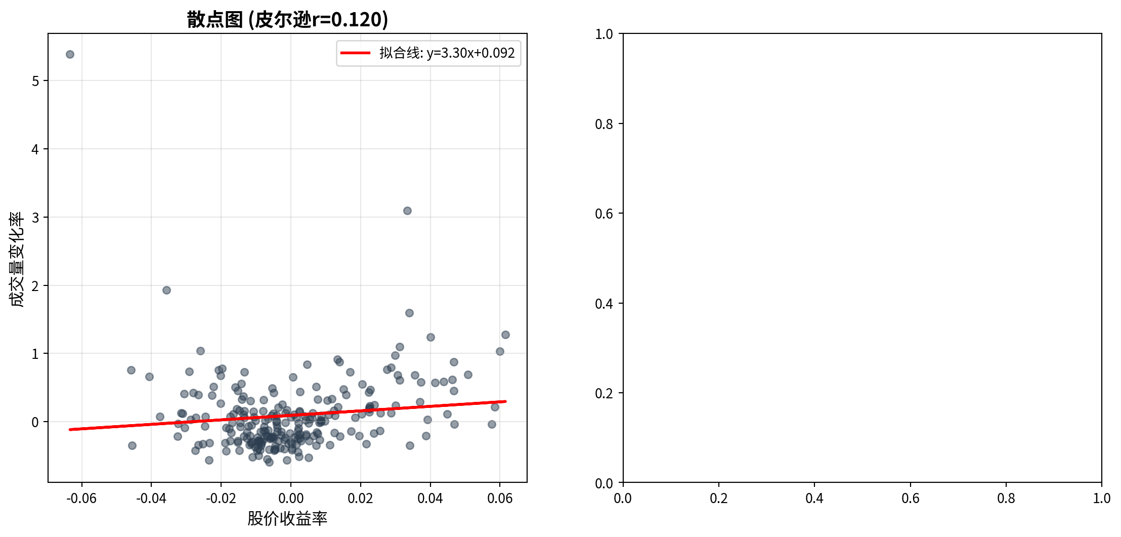
左侧散点图展示了海康威视日收益率(横轴)与成交量变化率(纵轴)之间的分布关系。从图中可以观察到:数据点围绕拟合线呈较为分散的分布,拟合线的正斜率反映了皮尔逊相关系数 \(r = 0.119\) 的正向关联,但大量数据点远离拟合线,直观地印证了这一相关性较弱的统计结论。此外,散点图中成交量变化率的纵向分布范围远大于收益率的横向分布范围,与前述描述性统计中成交量波动率(57.10%)远高于收益率波动率(2.07%)的结论一致。
The left scatter plot displays the distributional relationship between Hikvision’s daily returns (horizontal axis) and volume change rates (vertical axis). From the chart, one can observe that data points are dispersed around the fitted line; the positive slope of the fitted line reflects the positive association of the Pearson correlation coefficient \(r = 0.119\), but many data points lie far from the fitted line, visually confirming the statistical conclusion of a weak correlation. Additionally, the vertical spread of volume change rates in the scatter plot is much larger than the horizontal spread of returns, consistent with the earlier descriptive statistics showing that volume volatility (57.10%) far exceeds return volatility (2.07%).
下面在右侧面板绘制累积时间序列对比图,以观察量价关系的动态演变。
Next, we plot the cumulative time series comparison in the right panel to observe the dynamic evolution of the price-volume relationship.
# ========== 第3步:右图——累积时间序列对比 ==========
# ========== Step 3: Right panel — Cumulative time series comparison ==========
matplot_axes_array[1].plot(range(trading_days_count), np.cumsum(daily_returns_array), linewidth=1.5, label='累积收益率', color='#E3120B')  # 绘制累积收益率曲线(红色)
# Plot cumulative return curve (red)
twin_axes_object = matplot_axes_array[1].twinx()               # 创建共享x轴的辅助y轴(双纵轴)
# Create a secondary y-axis sharing the same x-axis (dual y-axes)
twin_axes_object.plot(range(trading_days_count), np.cumsum(volume_changes_array), linewidth=1.5, label='累积成交量变化', color='#008080', alpha=0.7)  # 绘制累积成交量变化曲线(青色)
# Plot cumulative volume change curve (teal)

matplot_axes_array[1].set_xlabel('交易日', fontsize=12)                           # 设置x轴标签
# Set x-axis label
matplot_axes_array[1].set_ylabel('累积收益率', fontsize=12, color='#E3120B')       # 左y轴标签(红色对应收益率)
# Left y-axis label (red for returns)
twin_axes_object.set_ylabel('累积成交量变化', fontsize=12, color='#008080')        # 右y轴标签(青色对应成交量)
# Right y-axis label (teal for volume)
matplot_axes_array[1].set_title('时间序列对比', fontsize=14, fontweight='bold')    # 设置子图标题
# Set subplot title

# ========== 第4步:合并双纵轴图例 ==========
# ========== Step 4: Merge dual y-axis legends ==========
plot_lines_primary, plot_labels_primary = matplot_axes_array[1].get_legend_handles_labels()      # 获取主y轴的图例句柄和标签
# Get legend handles and labels for the primary y-axis
plot_lines_secondary, plot_labels_secondary = twin_axes_object.get_legend_handles_labels()        # 获取辅助y轴的图例句柄和标签
# Get legend handles and labels for the secondary y-axis
matplot_axes_array[1].legend(plot_lines_primary + plot_lines_secondary, plot_labels_primary + plot_labels_secondary, loc='best', fontsize=10)  # 合并后显示在最佳位置
# Merge and display at the best position

matplot_axes_array[1].tick_params(axis='y', labelcolor='#E3120B')   # 左y轴刻度标签设为红色
# Set left y-axis tick labels to red
twin_axes_object.tick_params(axis='y', labelcolor='#008080')        # 右y轴刻度标签设为青色
# Set right y-axis tick labels to teal
matplot_axes_array[1].grid(True, alpha=0.3)                         # 添加半透明网格线
# Add semi-transparent gridlines

plt.tight_layout()  # 自动调整子图间距
# Automatically adjust subplot spacing
plt.show()          # 显示图形
# Display the figure
<Figure size 672x480 with 0 Axes>图 8.1 的右侧面板展示了累积收益率与累积成交量变化的时间序列对比。从图中可以观察到:累积收益率曲线(红色)在2023年全年呈现先升后降再趋稳的走势,而累积成交量变化曲线(青色)则呈现持续上升的趋势。两条曲线的走势并非严格同步——在某些阶段(如年初),两者方向一致;但在另一些阶段则出现明显分歧。这种不完全同步的动态关系印证了前文皮尔逊相关系数仅为0.12的弱线性关联结论,同时也暗示了量价关系可能具有时变特征,即在不同市场环境下关联强度会发生变化。
The right panel of 图 8.1 displays the time series comparison of cumulative returns and cumulative volume changes. From the chart, one can observe that the cumulative return curve (red) exhibits a pattern of rising first, then declining, and finally stabilizing throughout 2023, while the cumulative volume change curve (teal) shows a persistently upward trend. The trajectories of the two curves are not strictly synchronized—in some phases (such as early in the year), both move in the same direction; but in other phases, they diverge noticeably. This imperfectly synchronized dynamic relationship confirms the earlier conclusion of a weak linear association with a Pearson correlation coefficient of only 0.12, and also suggests that the price-volume relationship may have time-varying characteristics, meaning that the strength of association changes under different market conditions.
8.2.6 其他类型的相关系数 (Other Types of Correlation Coefficients)
除了皮尔逊相关系数,还有其他类型的相关度量:
Besides the Pearson correlation coefficient, there are other types of correlation measures:
1. 斯皮尔曼等级相关系数(Spearman’s ρ)
1. Spearman’s Rank Correlation Coefficient (Spearman’s ρ)
斯皮尔曼相关系数衡量两个变量之间的单调关系(不必线性),其计算基于数据的秩次而非原始值。设 \(d_i\) 为第 \(i\) 个观测值在两个变量上的秩次之差,则:
The Spearman correlation coefficient measures the monotonic relationship (not necessarily linear) between two variables. Its calculation is based on the ranks of the data rather than the raw values. Let \(d_i\) be the difference in ranks of the \(i\)-th observation across the two variables, then:
\[ \rho_s = 1 - \frac{6\sum_{i=1}^{n} d_i^2}{n(n^2-1)} \tag{8.5}\]
对异常值稳健
适用范围更广(有序变量也可)
Robust to outliers
Broader applicability (also applicable to ordinal variables)
2. 肯德尔τ系数(Kendall’s Tau)
2. Kendall’s Tau Coefficient (Kendall’s τ)
肯德尔τ系数基于秩的一致性(concordant)和不一致性(discordant)对数。设 \(C\) 为一致对数,\(D\) 为不一致对数,则:
Kendall’s τ coefficient is based on the number of concordant and discordant pairs of ranks. Let \(C\) be the number of concordant pairs and \(D\) the number of discordant pairs, then:
\[ \tau = \frac{C - D}{\binom{n}{2}} = \frac{C - D}{n(n-1)/2} \tag{8.6}\]
样本量较小时更准确
对异常值稳健
More accurate with small sample sizes
Robust to outliers
选择建议:
- 数据正态且线性关系 → 皮尔逊
- 数据非正态或存在异常值 → 斯皮尔曼或肯德尔
Selection guidelines:
- Data is normally distributed with a linear relationship → Pearson
- Data is non-normal or contains outliers → Spearman or Kendall ## 简单线性回归 (Simple Linear Regression) {#sec-simple-regression}
8.2.7 理论背景 (Theoretical Background)
简单线性回归(Simple Linear Regression)用于建模两个连续变量之间的线性关系。它是所有回归分析的基础,也是理解多元回归、非线性回归的起点。
Simple Linear Regression is used to model the linear relationship between two continuous variables. It is the foundation of all regression analysis and the starting point for understanding multiple regression and nonlinear regression.
模型设定(式 8.7):
Model Specification (式 8.7):
\[ Y_i = \beta_0 + \beta_1 X_i + \varepsilon_i \tag{8.7}\]
其中: - \(Y_i\):因变量(响应变量)的第 \(i\) 个观测值 - \(X_i\):自变量(解释变量)的第 \(i\) 个观测值 - \(\beta_0\):截距项(当 \(X=0\) 时 \(Y\) 的期望值) - \(\beta_1\):斜率系数(\(X\) 每增加1单位,\(Y\) 的期望变化量) - \(\varepsilon_i\):误差项(随机扰动)
Where: - \(Y_i\): The \(i\)-th observation of the dependent (response) variable - \(X_i\): The \(i\)-th observation of the independent (explanatory) variable - \(\beta_0\): The intercept (expected value of \(Y\) when \(X=0\)) - \(\beta_1\): The slope coefficient (expected change in \(Y\) per unit increase in \(X\)) - \(\varepsilon_i\): The error term (random disturbance)
经典假设(Gauss-Markov假设):
Classical Assumptions (Gauss-Markov Assumptions):
线性性:\(Y\) 与 \(X\) 的关系是线性的
外生性:\(E[\varepsilon_i | X_i] = 0\) (误差项条件期望为零)
同方差性:\(\text{Var}(\varepsilon_i | X_i) = \sigma^2\) (误差方差恒定)
无自相关:\(\text{Cov}(\varepsilon_i, \varepsilon_j) = 0\) for \(i \neq j\)
正态性(可选,用于推断):\(\varepsilon_i \sim N(0, \sigma^2)\)
Linearity: The relationship between \(Y\) and \(X\) is linear
Exogeneity: \(E[\varepsilon_i | X_i] = 0\) (the conditional expectation of the error term is zero)
Homoscedasticity: \(\text{Var}(\varepsilon_i | X_i) = \sigma^2\) (constant error variance)
No Autocorrelation: \(\text{Cov}(\varepsilon_i, \varepsilon_j) = 0\) for \(i \neq j\)
Normality (optional, for inference): \(\varepsilon_i \sim N(0, \sigma^2)\)
为什么要这些假设?
Why Are These Assumptions Needed?
线性性:简化模型,便于解释和计算
外生性:确保OLS估计量无偏
同方差性:确保OLS估计量有效(方差最小)
无自相关:确保标准误估计正确
正态性:使得小样本推断(t检验、F检验)有效
Linearity: Simplifies the model, facilitating interpretation and computation
Exogeneity: Ensures the OLS estimator is unbiased
Homoscedasticity: Ensures the OLS estimator is efficient (minimum variance)
No Autocorrelation: Ensures correct standard error estimation
Normality: Enables valid small-sample inference (t-tests, F-tests)
如果某些假设不满足,我们可能需要使用广义最小二乘法(GLS)、稳健标准误或其他方法。
If some assumptions are violated, we may need to use Generalized Least Squares (GLS), robust standard errors, or other methods.
8.2.8 最小二乘估计 (OLS) 的数学与几何 (Mathematics and Geometry of OLS Estimation)
普通最小二乘法 (OLS) 寻找一组参数 \(\beta\),使得预测误差的平方和最小。
Ordinary Least Squares (OLS) seeks a set of parameters \(\beta\) that minimizes the sum of squared prediction errors.
数学推导 (Matrix Calculus): 将模型写成矩阵形式 \(Y = X\beta + \varepsilon\)。残差平方和为:
Mathematical Derivation (Matrix Calculus): Write the model in matrix form \(Y = X\beta + \varepsilon\). The residual sum of squares is:
\[ SSE(\beta) = (Y - X\beta)^T (Y - X\beta) = Y^TY - 2\beta^T X^T Y + \beta^T X^T X \beta \]
对 \(\beta\) 求导并令其为 0:
Taking the derivative with respect to \(\beta\) and setting it to zero:
\[ \frac{\partial SSE}{\partial \beta} = -2X^T Y + 2X^T X \beta = 0 \]
整理得到正规方程 (Normal Equations):
Rearranging yields the Normal Equations:
\[ (X^T X) \beta = X^T Y \]
假设 \(X^T X\) 可逆,得到 OLS 估计量:
Assuming \(X^T X\) is invertible, we obtain the OLS estimator:
\[ \hat{\beta}_{OLS} = (X^T X)^{-1} X^T Y \]
几何解释 (Orthogonal Projection): 想象 \(Y\) 是 \(n\) 维空间中的一个向量。\(X\) 的列向量张成了一个子空间 (Subspace)。 回归问题实际上是寻找子空间中距离 \(Y\) 最近的向量 \(\hat{Y}\)。 根据几何原理,最短距离对应垂线。因此,残差向量 \(\varepsilon = Y - \hat{Y}\) 必须垂直于(正交于) \(X\) 张成的子空间。 这意味着 \(X^T (Y - X\hat{\beta}) = 0\),再次导出了正规方程。
Geometric Interpretation (Orthogonal Projection): Imagine \(Y\) as a vector in \(n\)-dimensional space. The column vectors of \(X\) span a subspace. The regression problem is essentially finding the vector \(\hat{Y}\) in that subspace closest to \(Y\). By geometric principles, the shortest distance corresponds to the perpendicular. Therefore, the residual vector \(\varepsilon = Y - \hat{Y}\) must be perpendicular (orthogonal) to the subspace spanned by \(X\). This means \(X^T (Y - X\hat{\beta}) = 0\), which again leads to the normal equations.
OLS 本质上就是一种正交投影 (Orthogonal Projection),将复杂的高维数据投影到我们能理解的低维模型空间上。
OLS is essentially an orthogonal projection, projecting complex high-dimensional data onto a lower-dimensional model space that we can understand.
斜率和截距的解析解分别如 式 8.8 和 式 8.9 所示:
The analytical solutions for the slope and intercept are shown in 式 8.8 and 式 8.9, respectively:
\[ \hat{\beta}_1 = \frac{\sum_{i=1}^{n}(X_i - \bar{X})(Y_i - \bar{Y})}{\sum_{i=1}^{n}(X_i - \bar{X})^2} \tag{8.8}\]
\[ \hat{\beta}_0 = \bar{Y} - \hat{\beta}_1 \bar{X} \tag{8.9}\]
几何解释: - \(\hat{\beta}_1\) 是协方差与 \(X\) 方差的比值 - 回归线必定通过点 \((\bar{X}, \bar{Y})\) - OLS使残差之和为零:\(\sum_{i=1}^n \hat{\varepsilon}_i = 0\)
Geometric Interpretation: - \(\hat{\beta}_1\) is the ratio of the covariance to the variance of \(X\) - The regression line must pass through the point \((\bar{X}, \bar{Y})\) - OLS ensures the sum of residuals equals zero: \(\sum_{i=1}^n \hat{\varepsilon}_i = 0\)
OLS估计量的性质:
Properties of the OLS Estimator:
在Gauss-Markov假设下,OLS估计量是BLUE: - Best(最小方差) - Linear(线性估计量) - Unbiased(无偏) - Estimator(估计量)
Under the Gauss-Markov assumptions, the OLS estimator is BLUE: - Best (minimum variance) - Linear (a linear estimator) - Unbiased - Estimator
8.2.9 回归模型的质量评估 (Quality Assessment of Regression Models)
8.2.9.1 决定系数 \(R^2\) (Coefficient of Determination \(R^2\))
\[ R^2 = \frac{\text{SSR}}{\text{SST}} = 1 - \frac{\text{SSE}}{\text{SST}} \tag{8.10}\]
其中: - \(\text{SST} = \sum_{i=1}^{n}(Y_i - \bar{Y})^2\) (总平方和) - \(\text{SSR} = \sum_{i=1}^{n}(\hat{Y}_i - \bar{Y})^2\) (回归平方和) - \(\text{SSE} = \sum_{i=1}^{n}(Y_i - \hat{Y}_i)^2\) (残差平方和)
Where: - \(\text{SST} = \sum_{i=1}^{n}(Y_i - \bar{Y})^2\) (Total Sum of Squares) - \(\text{SSR} = \sum_{i=1}^{n}(\hat{Y}_i - \bar{Y})^2\) (Regression Sum of Squares) - \(\text{SSE} = \sum_{i=1}^{n}(Y_i - \hat{Y}_i)^2\) (Error/Residual Sum of Squares)
解释:由 式 10.6 可知,\(R^2\) 表示模型解释的 \(Y\) 变异比例,取值范围 \([0, 1]\)。
Interpretation: As shown in 式 10.6, \(R^2\) represents the proportion of total variation in \(Y\) explained by the model, ranging from \([0, 1]\).
关于 \(R^2\) 的误解
Common Misconceptions About \(R^2\)
误解1:“\(R^2\) 越高,模型越好” - 正确理解:高 \(R^2\) 不一定意味着模型因果正确或预测准确。可能存在过拟合。
Misconception 1: “The higher the \(R^2\), the better the model” - Correct Understanding: A high \(R^2\) does not necessarily mean the model is causally correct or predictively accurate. Overfitting may be present.
误解2:“\(R^2\) 低意味着模型无用” - 正确理解:在社会科学中,\(R^2 = 0.2\) 可能已经很有价值。关键看理论是否合理、系数是否有意义。
Misconception 2: “A low \(R^2\) means the model is useless” - Correct Understanding: In the social sciences, \(R^2 = 0.2\) may already be quite valuable. What matters is whether the theory is sound and the coefficients are meaningful.
误解3:“\(R^2\) 可以直接比较不同模型” - 正确理解:只有当因变量相同时,\(R^2\) 才可比较。对于不同因变量,应使用其他标准(如AIC、BIC)。
Misconception 3: “\(R^2\) can be directly compared across different models” - Correct Understanding: \(R^2\) is only comparable when the dependent variable is the same. For different dependent variables, other criteria (such as AIC, BIC) should be used.
8.2.9.2 回归标准误 (Standard Error of Regression)
\[ s_e = \sqrt{\frac{\text{SSE}}{n-2}} \tag{8.11}\]
解释:由 式 8.11 可知,\(s_e\) 估计误差项的标准差 \(\sigma\),衡量观测值围绕回归线的离散程度。
Interpretation: As shown in 式 8.11, \(s_e\) estimates the standard deviation \(\sigma\) of the error term, measuring the dispersion of observations around the regression line.
8.2.9.3 系数的显著性检验 (Significance Test for Coefficients)
检验斜率系数是否显著不为零(式 8.12):
Testing whether the slope coefficient is significantly different from zero (式 8.12):
\[ t = \frac{\hat{\beta}_1 - 0}{\text{SE}(\hat{\beta}_1)} \tag{8.12}\]
其中标准误如 式 8.13 所定义:
Where the standard error is defined in 式 8.13:
\[ \text{SE}(\hat{\beta}_1) = \frac{s_e}{\sqrt{\sum_{i=1}^{n}(X_i - \bar{X})^2}} \tag{8.13}\]
\(t\) 统计量服从自由度为 \(n-2\) 的t分布。
The \(t\) statistic follows a t-distribution with \(n-2\) degrees of freedom.
回归系数的置信区间(式 8.14):
Confidence interval for the regression coefficient (式 8.14):
\[ \hat{\beta}_1 \pm t_{\alpha/2, n-2} \cdot \text{SE}(\hat{\beta}_1) \tag{8.14}\]
8.2.10 残差诊断 (Residual Diagnostics)
回归模型的可靠性取决于假设是否满足。残差分析是检验假设的重要工具。
The reliability of a regression model depends on whether its assumptions are satisfied. Residual analysis is an important tool for checking these assumptions.
1. 线性性检验 - 绘制残差 vs. 拟合值图 - 如果呈现随机散布,线性假设合理 - 如果呈现系统模式(如U型),可能需要非线性项
1. Linearity Check - Plot residuals vs. fitted values - If the pattern is random scatter, the linearity assumption is reasonable - If a systematic pattern appears (e.g., U-shaped), nonlinear terms may be needed
2. 同方差性检验 - 绘制残差 vs. 拟合值图 - 如果残差扩散程度恒定,同方差假设满足 - 如果呈现漏斗状,存在异方差
2. Homoscedasticity Check - Plot residuals vs. fitted values - If the spread of residuals is constant, the homoscedasticity assumption holds - If a funnel shape appears, heteroscedasticity is present
3. 正态性检验 - 绘制残差的QQ图(Q-Q Plot) - 如果点近似落在对角线上,正态假设合理 - 或使用Shapiro-Wilk检验
3. Normality Check - Plot a Q-Q plot of the residuals - If points approximately fall on the diagonal line, the normality assumption is reasonable - Alternatively, use the Shapiro-Wilk test
4. 独立性检验 - 绘制残差的时间序列图 - 或使用Durbin-Watson检验
4. Independence Check - Plot a time series plot of the residuals - Or use the Durbin-Watson test
8.3 从理论到实践:苦活累活 (From Theory to Practice: The “Dirty Work”)
在教科书中,线性回归是完美的。但在现实世界(尤其是金融市场)中,它充满了陷阱。
In textbooks, linear regression is perfect. But in the real world (especially in financial markets), it is full of pitfalls.
8.3.1 伪回归 (Spurious Regression)
假设你让两个醉汉在街上随机游荡(随机游走),记录他们的路径。你会惊讶地发现,他们的路径之间往往有”显著”的相关性(\(R^2 > 0.8\))!
Suppose you let two drunkards wander randomly on the street (random walks) and record their paths. You would be surprised to find that their paths often show “significant” correlation (\(R^2 > 0.8\))!
原理:这是时间序列分析中的经典陷阱。当两个时间序列都是非平稳(Non-stationary)的(如股价、GDP),它们随时间都有共同的趋势。
后果:直接回归会导致荒谬的结论。Granger 和 Newbold (1974) 证明了这一点。
对策:对数据进行差分(Differencing),即使用”收益率”而不是”价格”进行回归。
Mechanism: This is a classic trap in time series analysis. When two time series are both non-stationary (e.g., stock prices, GDP), they share a common trend over time.
Consequence: Direct regression leads to absurd conclusions. Granger and Newbold (1974) demonstrated this.
Remedy: Difference the data—that is, regress on “returns” rather than “prices.”
8.3.2 异方差与稳健标准误 (Heteroscedasticity and Robust Standard Errors)
在理想的 OLS 世界里,每个样本的误差方差都一样 (\(\text{Var}(\varepsilon_i) = \sigma^2\))。但在现实(尤其是金融数据)中,大公司的营收波动(方差)通常远大于小公司。
In the ideal OLS world, the error variance is the same for every observation (\(\text{Var}(\varepsilon_i) = \sigma^2\)). But in reality (especially with financial data), the revenue volatility (variance) of large firms is typically much greater than that of small firms.
异方差 (Heteroscedasticity):会导致 OLS 估计量依然无偏,但标准误 (\(SE\)) 失效,t 检验结果不可信。
解决方案:在 Python
statsmodels中,永远不要吝啬使用cov_type='HC3'或HC1。这会计算异方差稳健标准误 (Heteroscedasticity-Robust Standard Errors, White’s SE)。它就像给 t 检验穿上了一层防弹衣,即使存在异方差,推断依然有效。Heteroscedasticity: The OLS estimator remains unbiased, but the standard errors (\(SE\)) become invalid, making t-test results unreliable.
Solution: In Python’s
statsmodels, never hesitate to usecov_type='HC3'orHC1. This computes Heteroscedasticity-Robust Standard Errors (White’s SE). It is like putting a bulletproof vest on your t-tests—even when heteroscedasticity is present, inference remains valid.
8.3.3 案例:资产与营收关系(含稳健标准误) (Case Study: Asset–Revenue Relationship with Robust Standard Errors)
什么是企业规模与营收的回归分析?
What Is a Regression Analysis of Firm Size and Revenue?
公司的总资产规模与其营业收入之间通常存在正向关系:规模越大的企业,往往拥有更强的市场覆盖能力和更高的营收。但这种关系的强度如何?我们能否用总资产来预测营收?这对于企业估值、行业对标和投资分析都有实际意义。
There is typically a positive relationship between a company’s total asset size and its operating revenue: larger firms tend to have stronger market coverage and higher revenues. But how strong is this relationship? Can we use total assets to predict revenue? This has practical significance for corporate valuation, industry benchmarking, and investment analysis.
简单线性回归是探索两个定量变量之间线性关系的基础工具。但在实际财务数据中,不同规模企业的误差方差往往不等(异方差问题),这会导致普通OLS的标准误失效。因此,我们使用异方差稳健标准误(HC3)来保证推断的可靠性。下面分析长三角地区上市公司总资产与营业收入的关系,回归结果如 图 8.2 所示。
Simple linear regression is the fundamental tool for exploring the linear relationship between two quantitative variables. However, in real financial data, the error variance often differs across firms of different sizes (the heteroscedasticity problem), which invalidates the standard errors from ordinary OLS. Therefore, we use heteroscedasticity-robust standard errors (HC3) to ensure reliable inference. Below we analyze the relationship between total assets and operating revenue for listed companies in the Yangtze River Delta region; the regression results are shown in 图 8.2.
# ========== 导入所需库 ==========
# ========== Import required libraries ==========
import numpy as np                                  # 数值计算库
# NumPy library for numerical computation
import pandas as pd                                 # 数据处理与分析库
# Pandas library for data manipulation and analysis
import matplotlib.pyplot as plt                     # 导入matplotlib绘图库
# Import matplotlib plotting library
from sklearn.linear_model import LinearRegression   # scikit-learn线性回归模型
# Linear regression model from scikit-learn
from scipy import stats                             # 统计分布和检验函数
# Statistical distributions and test functions from SciPy
import platform                                     # 系统平台检测库
# Platform detection library

# ========== 第1步:设置本地数据路径 ==========
# ========== Step 1: Set local data path ==========
if platform.system() == 'Windows':                  # 判断当前操作系统是否为Windows
# Check if the current OS is Windows
    data_path = 'C:/qiufei/data/stock'              # Windows平台下的股票数据路径
    # Stock data path on Windows
else:                                               # 否则为Linux平台
# Otherwise it is Linux
    data_path = '/home/ubuntu/r2_data_mount/qiufei/data/stock'  # Linux平台下的股票数据路径
    # Stock data path on Linux

# ========== 第2步:读取本地财务报表和公司基本信息数据 ==========
# ========== Step 2: Load local financial statement and company basic info data ==========
financial_statement_dataframe = pd.read_hdf(f'{data_path}/financial_statement.h5')  # 读取上市公司财务报表数据
# Read listed company financial statement data
stock_basic_info_dataframe = pd.read_hdf(f'{data_path}/stock_basic_data.h5')        # 读取上市公司基本信息数据
# Read listed company basic information data
财务报表和公司基本信息数据加载完毕。下面筛选长三角地区上市公司并准备回归分析数据。
Financial statement and company basic information data have been loaded. Next, we filter listed companies in the Yangtze River Delta region and prepare the data for regression analysis.
# ========== 第3步:筛选长三角地区上市公司 ==========
# ========== Step 3: Filter listed companies in the YRD region ==========
yrd_provinces_list = ['上海市', '浙江省', '江苏省']  # 定义长三角三省市列表
# Define the list of three YRD provinces/municipalities
yrd_stock_codes_list = stock_basic_info_dataframe[stock_basic_info_dataframe['province'].isin(yrd_provinces_list)]['order_book_id'].tolist()  # 提取长三角公司股票代码列表
# Extract the list of stock codes for YRD companies

# ========== 第4步:筛选最新年报数据 ==========
# ========== Step 4: Filter the latest annual report data ==========
yrd_financial_dataframe = financial_statement_dataframe[financial_statement_dataframe['order_book_id'].isin(yrd_stock_codes_list)].copy()  # 筛选长三角公司的财务数据
# Filter financial data for YRD companies
yrd_financial_dataframe = yrd_financial_dataframe[yrd_financial_dataframe['quarter'].str.endswith('q4')]  # 仅保留第四季度年报数据
# Keep only Q4 annual report data
yrd_financial_dataframe = yrd_financial_dataframe.sort_values('quarter', ascending=False)  # 按季度降序排列(最新在前)
# Sort by quarter in descending order (latest first)
yrd_financial_dataframe = yrd_financial_dataframe.drop_duplicates(subset='order_book_id', keep='first')  # 每家公司保留最新年报
# Keep only the latest annual report for each company

# ========== 第5步:提取总资产和营业收入并转换单位 ==========
# ========== Step 5: Extract total assets and revenue, convert units ==========
yrd_financial_dataframe = yrd_financial_dataframe[['order_book_id', 'total_assets', 'revenue']].dropna()  # 提取关键字段并删除缺失值
# Extract key fields and drop missing values
yrd_financial_dataframe['total_assets_billion'] = yrd_financial_dataframe['total_assets'] / 1e8  # 将总资产从元转换为亿元
# Convert total assets from CNY to hundred millions (yi yuan)
yrd_financial_dataframe['revenue_billion'] = yrd_financial_dataframe['revenue'] / 1e8            # 将营业收入从元转换为亿元
# Convert revenue from CNY to hundred millions (yi yuan)

# ========== 第6步:过滤极端值 ==========
# ========== Step 6: Filter extreme values ==========
yrd_financial_dataframe = yrd_financial_dataframe[(yrd_financial_dataframe['total_assets_billion'] > 1) & (yrd_financial_dataframe['total_assets_billion'] < 5000)]  # 总资产筛选范围:1~5000亿元
# Total assets filter range: 1–5000 hundred million yuan
yrd_financial_dataframe = yrd_financial_dataframe[(yrd_financial_dataframe['revenue_billion'] > 0) & (yrd_financial_dataframe['revenue_billion'] < 1000)]            # 营业收入筛选范围:>0且<1000亿元
# Revenue filter range: >0 and <1000 hundred million yuan

# ========== 第7步:拟合OLS线性回归模型 ==========
# ========== Step 7: Fit OLS linear regression model ==========
total_assets_billion_array = yrd_financial_dataframe['total_assets_billion'].values  # 提取总资产为NumPy数组(自变量X)
# Extract total assets as NumPy array (independent variable X)
revenue_billion_array = yrd_financial_dataframe['revenue_billion'].values            # 提取营业收入为NumPy数组(因变量Y)
# Extract revenue as NumPy array (dependent variable Y)

independent_variable_matrix = total_assets_billion_array.reshape(-1, 1)  # 将自变量转为列向量(sklearn要求二维输入)
# Reshape independent variable to column vector (sklearn requires 2D input)
dependent_variable_array = revenue_billion_array                         # 因变量为一维数组
# Dependent variable as a 1D array
数据准备完成后,下面我们拟合OLS线性回归模型,计算截距、斜率、决定系数 \(R^2\)、系数的t统计量和置信区间等回归统计量,并对模型结果进行经济学解释。
After data preparation, we now fit the OLS linear regression model, compute the intercept, slope, coefficient of determination \(R^2\), t-statistics and confidence intervals for the coefficients, and provide economic interpretation of the model results.
linear_regression_model = LinearRegression()                             # 实例化线性回归模型
# Instantiate the linear regression model
linear_regression_model.fit(independent_variable_matrix, dependent_variable_array)  # 拟合模型:最小化残差平方和
# Fit the model: minimize the residual sum of squares
estimated_intercept_beta0 = linear_regression_model.intercept_           # 提取截距估计值β₀
# Extract the estimated intercept β₀
estimated_slope_beta1 = linear_regression_model.coef_[0]                 # 提取斜率估计值β₁
# Extract the estimated slope β₁
predicted_revenue_array = linear_regression_model.predict(independent_variable_matrix)  # 计算拟合值(预测营业收入)
# Compute fitted values (predicted revenue)
regression_residuals_array = dependent_variable_array - predicted_revenue_array          # 计算残差 = 实际值 - 拟合值
# Compute residuals = actual values - fitted values

# ========== 第8步:计算回归统计量 ==========
# ========== Step 8: Compute regression statistics ==========
sample_size_count = len(dependent_variable_array)                        # 样本量
# Sample size
mean_revenue_value = np.mean(dependent_variable_array)                   # 因变量(营业收入)均值
# Mean of the dependent variable (revenue)
total_sum_of_squares = np.sum((dependent_variable_array - mean_revenue_value)**2)    # SST:总平方和,衡量Y的总离散程度
# SST: Total Sum of Squares, measuring total dispersion of Y
error_sum_of_squares = np.sum(regression_residuals_array**2)             # SSE:残差平方和,衡量模型未解释的离散
# SSE: Error Sum of Squares, measuring unexplained dispersion
regression_sum_of_squares = np.sum((predicted_revenue_array - mean_revenue_value)**2)  # SSR:回归平方和,衡量模型解释的离散
# SSR: Regression Sum of Squares, measuring explained dispersion

# 计算决定系数R²
# Compute the coefficient of determination R²
r_squared_value = 1 - error_sum_of_squares / total_sum_of_squares        # R² = 1 - SSE/SST,衡量模型拟合优度
# R² = 1 - SSE/SST, measuring goodness of fit

# 计算回归标准误
# Compute the regression standard error
regression_standard_error = np.sqrt(error_sum_of_squares / (sample_size_count - 2))  # 回归标准误 = sqrt(SSE/(n-2)),估计σ
# Regression standard error = sqrt(SSE/(n-2)), estimating σ
回归统计量(SST、SSE、SSR、R²、标准误)计算完毕。下面计算系数的标准误、t统计量和置信区间。
The regression statistics (SST, SSE, SSR, R², standard error) have been computed. Next we compute the standard errors, t-statistics, and confidence intervals for the coefficients.
# ========== 第9步:计算系数标准误、t统计量和置信区间 ==========
# ========== Step 9: Compute coefficient standard errors, t-statistics, and confidence intervals ==========
standard_error_beta1 = regression_standard_error / np.sqrt(np.sum((total_assets_billion_array - np.mean(total_assets_billion_array))**2))  # β₁的标准误 = s_e / sqrt(Σ(Xi-X̄)²)
# Standard error of β₁ = s_e / sqrt(Σ(Xi-X̄)²)
standard_error_beta0 = regression_standard_error * np.sqrt(1/sample_size_count + (np.mean(total_assets_billion_array)**2) / np.sum((total_assets_billion_array - np.mean(total_assets_billion_array))**2))  # β₀的标准误
# Standard error of β₀

# 计算t统计量和双侧p值
# Compute t-statistics and two-sided p-values
t_statistic_beta1 = estimated_slope_beta1 / standard_error_beta1         # β₁的t统计量 = β̂₁/SE(β̂₁)
# t-statistic of β₁ = β̂₁/SE(β̂₁)
p_value_beta1 = 2 * (1 - stats.t.cdf(abs(t_statistic_beta1), df=sample_size_count-2))  # β₁的双侧p值
# Two-sided p-value of β₁

t_statistic_beta0 = estimated_intercept_beta0 / standard_error_beta0     # β₀的t统计量 = β̂₀/SE(β̂₀)
# t-statistic of β₀ = β̂₀/SE(β̂₀)
p_value_beta0 = 2 * (1 - stats.t.cdf(abs(t_statistic_beta0), df=sample_size_count-2))  # β₀的双侧p值
# Two-sided p-value of β₀

# 计算95%置信区间
# Compute 95% confidence intervals
critical_t_value = stats.t.ppf(0.975, df=sample_size_count-2)           # 求t分布97.5%分位数(双侧α=0.05的临界值)
# 97.5th percentile of the t-distribution (critical value for two-sided α=0.05)
confidence_interval_beta1 = (estimated_slope_beta1 - critical_t_value * standard_error_beta1, estimated_slope_beta1 + critical_t_value * standard_error_beta1)  # β₁的95%置信区间
# 95% confidence interval of β₁
confidence_interval_beta0 = (estimated_intercept_beta0 - critical_t_value * standard_error_beta0, estimated_intercept_beta0 + critical_t_value * standard_error_beta0)  # β₀的95%置信区间
# 95% confidence interval of β₀
完成回归统计量计算和系数检验后,我们输出完整的回归分析结果及其经济学解释:
After completing the regression statistics and coefficient tests, we output the full regression results along with their economic interpretation:
# ========== 第10步:输出描述性统计与回归结果 ==========
# ========== Step 10: Output descriptive statistics and regression results ==========
print('=' * 60)                                                          # 分隔线
# Separator line
print('长三角上市公司总资产与营业收入线性回归分析')                        # 标题
# Title
print('=' * 60)                                                          # 分隔线
# Separator line

print('\n描述性统计:')                                                    # 描述性统计标题
# Descriptive statistics header
print(f'  样本量: {sample_size_count}')                                   # 输出样本量
# Print sample size
print(f'  总资产 - 均值: {np.mean(total_assets_billion_array):.2f} 亿元, 标准差: {np.std(total_assets_billion_array, ddof=1):.2f} 亿元')  # 总资产的均值和标准差
# Mean and std dev of total assets
print(f'  营业收入 - 均值: {np.mean(revenue_billion_array):.2f} 亿元, 标准差: {np.std(revenue_billion_array, ddof=1):.2f} 亿元')          # 营业收入的均值和标准差
# Mean and std dev of revenue

print('\n' + '=' * 60)                                                   # 分隔线
# Separator line
print('回归结果')                                                         # 回归结果标题
# Regression results header
print('=' * 60)                                                          # 分隔线
# Separator line
print(f'\n拟合方程:')                                                     # 拟合方程标题
# Fitted equation header
print(f'  营业收入 = {estimated_intercept_beta0:.2f} + {estimated_slope_beta1:.2f} × 总资产')  # 输出回归方程
# Print the regression equation

print(f'\n截距 (β₀):')                                                   # 截距部分标题
# Intercept section header
print(f'  估计值: {estimated_intercept_beta0:.2f} 亿元')                  # 截距估计值
# Estimated intercept value
print(f'  标准误: {standard_error_beta0:.2f}')                            # 截距标准误
# Standard error of intercept
print(f'  t统计量: {t_statistic_beta0:.4f}')                              # 截距t统计量
# t-statistic of intercept
print(f'  p值: {p_value_beta0:.6f}')                                     # 截距p值
# p-value of intercept
print(f'  95% CI: [{confidence_interval_beta0[0]:.2f}, {confidence_interval_beta0[1]:.2f}]')  # 截距95%置信区间
# 95% confidence interval of intercept
============================================================
长三角上市公司总资产与营业收入线性回归分析
============================================================
描述性统计:
样本量: 1833
总资产 - 均值: 117.43 亿元, 标准差: 320.05 亿元
营业收入 - 均值: 50.67 亿元, 标准差: 108.51 亿元
============================================================
回归结果
============================================================
拟合方程:
营业收入 = 28.97 + 0.18 × 总资产
截距 (β₀):
估计值: 28.97 亿元
标准误: 2.26
t统计量: 12.7948
p值: 0.000000
95% CI: [24.53, 33.41]回归分析基于1833家长三角上市公司的数据(总资产均值117.43亿元、标准差320.05亿元;营业收入均值50.67亿元、标准差108.51亿元),拟合方程为:营业收入 = 28.97 + 0.18 × 总资产。截距 \(\hat{\beta}_0 = 28.97\) 亿元,t统计量为12.7948,p值接近于零(0.000000),在任何常用显著性水平下均高度显著,95%置信区间为[24.53, 33.41]亿元。截距的经济含义是:当总资产为零时,营业收入的预期值约为29亿元——虽然”零资产”在实际中不存在,但截距保证了回归线在数据范围内的拟合精度。
The regression analysis is based on data from 1,833 listed companies in the Yangtze River Delta (mean total assets: 117.43 hundred million yuan, std dev: 320.05; mean revenue: 50.67 hundred million yuan, std dev: 108.51). The fitted equation is: Revenue = 28.97 + 0.18 × Total Assets. The intercept \(\hat{\beta}_0 = 28.97\) hundred million yuan, with a t-statistic of 12.7948 and a p-value close to zero (0.000000), is highly significant at any conventional significance level, with a 95% confidence interval of [24.53, 33.41]. The economic meaning of the intercept is: when total assets are zero, the expected revenue is approximately 29 hundred million yuan—although “zero assets” does not exist in practice, the intercept ensures the accuracy of the regression line’s fit within the data range.
下面输出斜率系数的估计与推断结果及模型拟合度。
Below we output the estimation and inference results for the slope coefficient and the model’s goodness of fit.
print(f'\n斜率 (β₁):')                                                  # 输出斜率参数标题
# Slope parameter header
print(f'  估计值: {estimated_slope_beta1:.4f} (每亿元资产带来的营业收入)')  # 输出斜率估计值及经济含义
# Estimated slope value and economic meaning
print(f'  标准误: {standard_error_beta1:.4f}')                             # 输出斜率标准误差
# Standard error of slope
print(f'  t统计量: {t_statistic_beta1:.4f}')                              # 输出斜率t检验统计量
# t-statistic of slope
print(f'  p值: {p_value_beta1:.6f}')                                      # 斜率p值
# p-value of slope
print(f'  95% CI: [{confidence_interval_beta1[0]:.4f}, {confidence_interval_beta1[1]:.4f}]')  # 斜率95%置信区间
# 95% confidence interval of slope

print(f'\n模型拟合度:')                                                   # 模型拟合度标题
# Model goodness of fit header
print(f'  R²: {r_squared_value:.4f}')                                    # 输出R²(决定系数)
# Print R² (coefficient of determination)
print(f'  回归标准误: {regression_standard_error:.2f} 亿元')              # 输出回归标准误
# Print regression standard error
print(f'  解释: 总资产解释了营业收入变异的{r_squared_value*100:.1f}%')    # R²的直观解释
# Interpretation: total assets explain this percentage of revenue variation
斜率 (β₁):
  估计值: 0.1848 (每亿元资产带来的营业收入)
  标准误: 0.0066
  t统计量: 27.8089
  p值: 0.000000
  95% CI: [0.1717, 0.1978]

模型拟合度:
  R²: 0.2969
  回归标准误: 91.01 亿元
  解释: 总资产解释了营业收入变异的29.7%
斜率系数 \(\hat{\beta}_1 = 0.1848\),标准误为0.0066,t统计量高达27.8089,p值为0.000000,95%置信区间为[0.1717, 0.1978]——斜率在统计上高度显著。其经济含义是:长三角地区上市公司的总资产每增加1亿元,营业收入平均增加约0.18亿元(即1848万元),或者说每100亿元的资产规模增长对应约18.48亿元的营业收入增量。模型的决定系数 \(R^2 = 0.2969\),表明总资产规模仅解释了营业收入变异的29.7%,回归标准误为91.01亿元。这一 \(R^2\) 值提示:虽然资产规模是影响营业收入的重要因素,但行业差异、经营效率、市场竞争等其他因素同样重要,实际应用中应考虑多元回归模型。
The slope coefficient \(\hat{\beta}_1 = 0.1848\), with a standard error of 0.0066, a t-statistic as high as 27.8089, a p-value of 0.000000, and a 95% confidence interval of [0.1717, 0.1978]—the slope is highly statistically significant. Its economic meaning is: for every additional 100 million yuan in total assets among YRD-listed companies, operating revenue increases by approximately 0.18 hundred million yuan (i.e., 18.48 million yuan), or equivalently, every 10 billion yuan increase in asset size corresponds to an increase of approximately 1.848 billion yuan in revenue. The coefficient of determination \(R^2 = 0.2969\), indicating that total asset size explains only 29.7% of the variation in operating revenue, with a regression standard error of 91.01 hundred million yuan. This \(R^2\) value suggests that although asset size is an important factor affecting revenue, other factors such as industry differences, operational efficiency, and market competition are equally important, and a multiple regression model should be considered in practice.
下面从经济学角度解释回归结果的实际意义,包括边际效应、模型预测和局限性分析。
Below we interpret the practical significance of the regression results from an economic perspective, including marginal effects, model predictions, and limitations analysis.
# ========== 第11步:输出实际意义解释 ==========
# ========== Step 11: Output practical significance interpretation ==========
print('\n' + '=' * 60)                                                   # 分隔线
# Separator line
print('实际意义解释')                                                     # 实际意义标题
# Practical significance header
print('=' * 60)                                                          # 分隔线
# Separator line
print(f'\n1. 斜率解释:')                                                  # 斜率经济含义
# Slope economic meaning
print(f'   总资产每增加1亿元,营业收入平均增加{estimated_slope_beta1:.4f}亿元')  # 边际效应解读
# Marginal effect interpretation
print(f'   95%置信区间为[{confidence_interval_beta1[0]:.4f}, {confidence_interval_beta1[1]:.4f}]亿元')  # 斜率区间估计
# Slope interval estimate

# ========== 第12步:模型预测与局限性说明 ==========
# ========== Step 12: Model prediction and limitations ==========
print(f'\n2. 模型预测:')                                                  # 模型预测标题
# Model prediction header
example_asset_billion = 100                                              # 设定一个示例总资产值(100亿元)
# Set an example total asset value (10 billion yuan)
example_predicted_revenue = estimated_intercept_beta0 + estimated_slope_beta1 * example_asset_billion  # 代入回归方程计算预测值
# Substitute into the regression equation to compute the predicted value
print(f'   预测:总资产{example_asset_billion}亿元的公司,营业收入约为{example_predicted_revenue:.2f}亿元')  # 输出点预测结果
# Print point prediction result

print(f'\n3. 模型局限性:')                                                # 模型局限性标题
# Model limitations header
print(f'   - R² = {r_squared_value:.4f},说明总资产只能解释部分营业收入变异')  # R²不高说明还有其他影响因素
# R² is not high, indicating other factors affect revenue
print(f'   - 其他重要因素:行业、经营效率、市场环境等')                    # 遗漏变量提示
# Omitted variable reminder
print(f'   - 实际应用中应使用多元回归模型')                                # 扩展建议:多元回归
# Extension suggestion: multiple regression
============================================================
实际意义解释
============================================================

1. 斜率解释:
   总资产每增加1亿元,营业收入平均增加0.1848亿元
   95%置信区间为[0.1717, 0.1978]亿元

2. 模型预测:
   预测:总资产100亿元的公司,营业收入约为47.45亿元

3. 模型局限性:
   - R² = 0.2969,说明总资产只能解释部分营业收入变异
   - 其他重要因素:行业、经营效率、市场环境等
   - 实际应用中应使用多元回归模型
8.3.4 回归诊断可视化 (Regression Diagnostics Visualization)
图 8.3 展示了回归模型的四幅诊断图。
图 8.3 presents four diagnostic plots for the regression model.
# ========== 第1步:创建2×2子图画布 ==========
# ========== Step 1: Create a 2×2 subplot canvas ==========
matplot_figure, matplot_axes_array = plt.subplots(2, 2, figsize=(14, 12))  # 创建2行2列的子图网格
# Create a 2-row, 2-column subplot grid

# ========== 第2步:面板A——散点图与回归线 ==========
# ========== Step 2: Panel A — Scatter plot with regression line ==========
matplot_axes_array[0, 0].scatter(total_assets_billion_array, revenue_billion_array, alpha=0.6, s=50, color='#2C3E50', label='观测数据')  # 绘制散点图(总资产 vs 营业收入)
# Plot scatter (total assets vs revenue)
matplot_axes_array[0, 0].plot(total_assets_billion_array, predicted_revenue_array, 'r-', linewidth=2.5, label=f'拟合线: y={estimated_intercept_beta0:.2f}+{estimated_slope_beta1:.2f}x')  # 叠加OLS回归线
# Overlay the OLS regression line
matplot_axes_array[0, 0].set_xlabel('总资产 (亿元)', fontsize=12)        # x轴标签:总资产
# x-axis label: Total Assets
matplot_axes_array[0, 0].set_ylabel('营业收入 (亿元)', fontsize=12)      # y轴标签:营业收入
# y-axis label: Revenue
matplot_axes_array[0, 0].set_title('(A) 散点图与回归线', fontsize=14, fontweight='bold')  # 面板标题
# Panel title
matplot_axes_array[0, 0].legend(fontsize=10)                             # 显示图例
# Display legend
matplot_axes_array[0, 0].grid(True, alpha=0.3)                           # 添加网格线
# Add gridlines

# ========== 第3步:面板B——残差vs拟合值图(检验线性性和同方差性) ==========
# ========== Step 3: Panel B — Residuals vs. fitted values (testing linearity and homoscedasticity) ==========
matplot_axes_array[0, 1].scatter(predicted_revenue_array, regression_residuals_array, alpha=0.6, s=50, color='#2C3E50')  # 绘制残差散点图
# Plot residual scatter
matplot_axes_array[0, 1].axhline(0, color='red', linestyle='--', linewidth=2)  # 添加y=0参考线(残差应围绕0分布)
# Add y=0 reference line (residuals should be centered around 0)
matplot_axes_array[0, 1].set_xlabel('拟合值', fontsize=12)               # x轴标签:模型拟合值
# x-axis label: Fitted values
matplot_axes_array[0, 1].set_ylabel('残差', fontsize=12)                 # y轴标签:残差
# y-axis label: Residuals
matplot_axes_array[0, 1].set_title('(B) 残差 vs. 拟合值 (检验线性性和同方差性)', fontsize=14, fontweight='bold')  # 面板标题
# Panel title
matplot_axes_array[0, 1].grid(True, alpha=0.3)                           # 添加网格线
# Add gridlines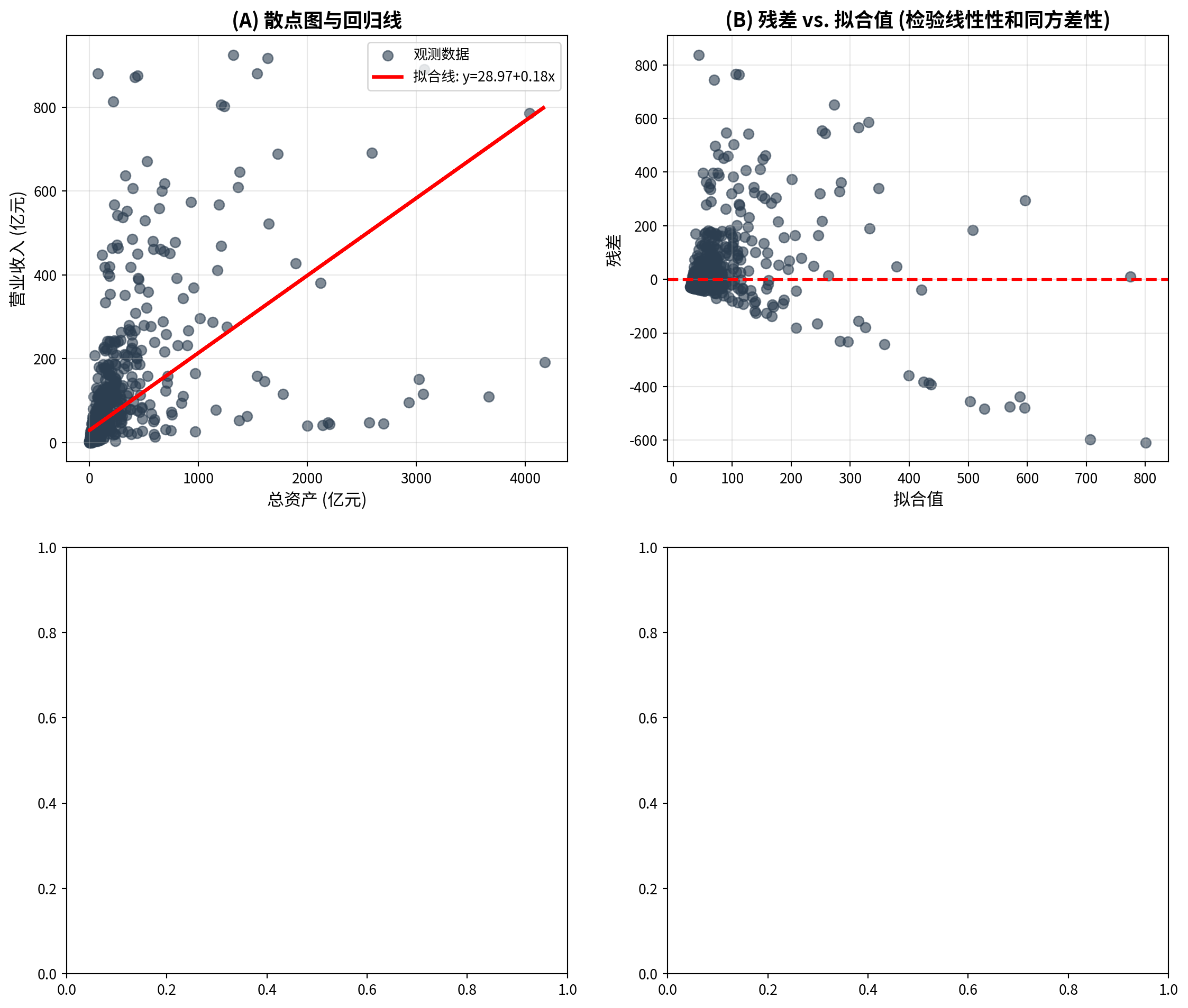
面板A展示了1833家长三角上市公司总资产与营业收入的散点图及OLS回归线,可以看到数据点在低总资产区域高度集中,而在高总资产区域稀疏分布,呈现明显的右偏特征。面板B的残差与拟合值图揭示了重要的诊断信息:残差在低拟合值处集中且方差较小,随着拟合值增大,残差的散布范围明显增大,呈现”喇叭形”扩散模式——这是异方差性(heteroscedasticity)的典型表现,意味着同方差假设可能不满足。此外,残差分布的不对称性提示数据中可能存在需要关注的非线性成分。
Panel A shows the scatter plot and OLS regression line for total assets versus operating revenue of 1,833 YRD-listed companies. The data points are highly concentrated in the low total asset region and sparsely distributed in the high total asset region, exhibiting a clear right-skewed pattern. The residuals-vs.-fitted-values plot in Panel B reveals important diagnostic information: residuals are concentrated with small variance at low fitted values, and the spread of residuals clearly increases as fitted values grow, displaying a “trumpet-shaped” expansion pattern — this is a typical manifestation of heteroscedasticity, indicating that the homoscedasticity assumption may not hold. Furthermore, the asymmetry in the residual distribution suggests that nonlinear components in the data may require attention.
下面绘制面板C(QQ图)和面板D(残差直方图),进一步检验正态性假设。
Below we plot Panel C (Q-Q plot) and Panel D (residual histogram) to further test the normality assumption.
# ========== 第4步:面板C——QQ图(检验残差正态性) ==========
# ========== Step 4: Panel C — Q-Q plot (testing residual normality) ==========
stats.probplot(regression_residuals_array, dist='norm', plot=matplot_axes_array[1, 0])  # 生成正态QQ图
# Generate normal Q-Q plot
matplot_axes_array[1, 0].set_title('(C) 残差QQ图 (检验正态性)', fontsize=14, fontweight='bold')  # 面板标题
# Panel title
matplot_axes_array[1, 0].grid(True, alpha=0.3)                           # 添加网格线
# Add gridlines

# ========== 第5步:面板D——残差直方图(观察残差分布形态) ==========
# ========== Step 5: Panel D — Residual histogram (observing residual distribution shape) ==========
matplot_axes_array[1, 1].hist(regression_residuals_array, bins=20, color='#008080', alpha=0.7, edgecolor='black')  # 绘制残差直方图
# Plot residual histogram
matplot_axes_array[1, 1].axvline(0, color='red', linestyle='--', linewidth=2)  # 添加x=0参考线
# Add x=0 reference line
matplot_axes_array[1, 1].set_xlabel('残差', fontsize=12)                 # x轴标签:残差
# x-axis label: Residuals
matplot_axes_array[1, 1].set_ylabel('频数', fontsize=12)                 # y轴标签:频数
# y-axis label: Frequency
matplot_axes_array[1, 1].set_title('(D) 残差分布直方图', fontsize=14, fontweight='bold')  # 面板标题
# Panel title
matplot_axes_array[1, 1].grid(True, alpha=0.3, axis='y')                 # 仅在y轴方向添加网格线
# Add gridlines on y-axis only

plt.tight_layout()                                                       # 自动调整子图间距
# Automatically adjust subplot spacing
plt.show()                                                               # 显示图形
# Display the figure
<Figure size 672x480 with 0 Axes>图 8.3 的四幅诊断图提供了模型假设检验的综合视角。面板C的QQ图显示残差在两端明显偏离45度对角线,尤其是右尾出现严重上翘,说明残差分布具有”厚尾”特征,正态性假设不能成立。面板D的残差直方图进一步证实了这一判断:直方图呈现显著的右偏形态,峰度高于正态分布(尖峰),且存在较多的正向极端残差。综合四幅诊断图的发现:(1) 异方差性明显(面板B的喇叭形);(2) 正态性不满足(面板C的尾部偏离和面板D的右偏分布)。这些问题提示:在对企业财务数据进行回归分析时,可能需要对数据进行对数变换,或使用稳健标准误(HC标准误)来获得可靠的统计推断。
The four diagnostic plots in 图 8.3 provide a comprehensive perspective on checking model assumptions. The Q-Q plot in Panel C shows that the residuals deviate markedly from the 45-degree diagonal at both tails, especially with severe upward curvature in the right tail, indicating that the residual distribution has “heavy tail” characteristics and the normality assumption cannot be sustained. The residual histogram in Panel D further confirms this finding: the histogram exhibits a pronounced right-skewed shape, with kurtosis higher than the normal distribution (leptokurtic), and a substantial number of large positive residuals. Combining the findings from all four diagnostic plots: (1) heteroscedasticity is evident (the trumpet shape in Panel B); (2) normality is not satisfied (the tail deviation in Panel C and the right-skewed distribution in Panel D). These issues suggest that when performing regression analysis on corporate financial data, a logarithmic transformation of the data may be needed, or robust standard errors (HC standard errors) should be used to obtain reliable statistical inference.
8.4 相关与回归的区别与联系 (Differences and Connections Between Correlation and Regression)
8.4.1 主要区别 (Key Differences)
| 特征 | 相关分析 | 回归分析 |
|---|---|---|
| 目的 | 衡量变量关联强度 | 预测或解释因变量 |
| 变量角色 | 对称,无因变量与自变量之分 | 不对称,区分因变量与自变量 |
| 取值范围 | \(-1\) 到 \(1\) | 系数可为任意实数 |
| 单位 | 无量纲 | 有单位 |
| 因果推断 | 不涉及 | 可用于因果分析(需满足假设) |
| Feature | Correlation Analysis | Regression Analysis |
|---|---|---|
| Purpose | Measure strength of association | Predict or explain the dependent variable |
| Variable Roles | Symmetric; no distinction between DV and IV | Asymmetric; distinguishes DV from IV |
| Range | \(-1\) to \(1\) | Coefficients can be any real number |
| Units | Dimensionless | Has units |
| Causal Inference | Not involved | Can be used for causal analysis (if assumptions hold) |
8.4.2 数值关系 (Numerical Relationship)
在简单线性回归中,相关系数与回归斜率有如 式 8.15 所示的关系:
In simple linear regression, the correlation coefficient and the regression slope have the relationship shown in 式 8.15:
\[ \hat{\beta}_1 = r \cdot \frac{s_Y}{s_X} \tag{8.15}\]
其中: - \(r\) 为皮尔逊相关系数 - \(s_Y, s_X\) 为样本标准差
Where: - \(r\) is the Pearson correlation coefficient - \(s_Y, s_X\) are the sample standard deviations
推论: - 如果 \(X\) 和 \(Y\) 标准化(均值为0,标准差为1),则 \(\hat{\beta}_1 = r\) - 决定系数 \(R^2 = r^2\) (在简单回归中)
Corollaries: - If \(X\) and \(Y\) are standardized (mean zero, standard deviation one), then \(\hat{\beta}_1 = r\) - The coefficient of determination \(R^2 = r^2\) (in simple regression)
8.4.3 选择建议 (Selection Advice)
使用相关分析: - 主要关注变量间的关联强度 - 不区分预测变量和响应变量 - 进行探索性数据分析
Use Correlation Analysis When: - The main focus is on the strength of association between variables - There is no distinction between predictor and response variables - Conducting exploratory data analysis
使用回归分析: - 需要预测或解释 - 需要控制其他变量(多元回归) - 关注因果机制
Use Regression Analysis When: - Prediction or explanation is needed - Other variables need to be controlled (multiple regression) - The focus is on causal mechanisms
8.4.4 启发式思考题 (Heuristic Problems)
1. 安斯库姆四重奏 (Anscombe’s Quartet) - 弗朗西斯·安斯库姆 (Francis Anscombe) 构造了四组数据,它们拥有完全相同的均值、方差、相关系数和回归线,但绘图后形态千差万别。 - Dataset I: 正常的线性关系。 - Dataset II: 完美的非线性(U型)关系,但线性回归强行拟合。 - Dataset III: 只有一个离群值拉歪了回归线。 - Dataset IV: \(X\) 几乎不变,全靠一个极端值撑起相关性。 - 任务:编写 Python 代码复现这四组数据,并计算 R2。这不仅是视觉冲击,更是对”盲目相信统计指标”的当头棒喝。
1. Anscombe’s Quartet - Francis Anscombe constructed four datasets that have exactly the same means, variances, correlation coefficients, and regression lines, yet look completely different when plotted. - Dataset I: A normal linear relationship. - Dataset II: A perfect nonlinear (U-shaped) relationship, but linear regression is forced to fit. - Dataset III: A single outlier skews the regression line. - Dataset IV: \(X\) is nearly constant; the correlation is entirely supported by one extreme point. - Task: Write Python code to reproduce these four datasets and compute R². This is not just a visual shock, but a powerful wake-up call against “blindly trusting statistical indicators.”
2. 厨房水槽回归 (The Kitchen Sink Regression) - 很多初学者认为 \(R^2\) 越高越好,所以把所有能找到的变量都塞进模型里(Everything including the kitchen sink)。 - 实验:生成一个只有噪声的 \(Y\),然后随机生成 100 个只有噪声的 \(X\)。 - 逐步将 \(X\) 加入回归模型。 - 观察:你会发现 \(R^2\) 单调递增,直到达到 1.0(当变量数=样本数时)。 - 反思:这也是为什么我们更看重 调整后 \(R^2\) (Adjusted \(R^2\)),它会惩罚那些对模型没有贡献的冗余变量。
2. The Kitchen Sink Regression - Many beginners believe the higher the \(R^2\), the better, so they stuff every available variable into the model (everything including the kitchen sink). - Experiment: Generate a \(Y\) that is pure noise, then randomly generate 100 noise-only \(X\) variables. - Progressively add the \(X\) variables into the regression model. - Observation: You will find that \(R^2\) monotonically increases, reaching 1.0 (when the number of variables equals the sample size). - Reflection: This is why we place greater emphasis on the Adjusted \(R^2\), which penalizes redundant variables that do not contribute to the model.
3. 对撞因子偏差 (Collider Bias) - 好莱坞明星往往”颜值高”和”演技好”呈负相关。难道老天是公平的? - 解释:只有”颜值高”或者”演技好”(或二者兼备)的人才能进入好莱坞(样本选择)。 - 任务:模拟两列独立的随机正态数据 \(A\) (颜值) 和 \(B\) (演技)。 - 选择 \(A+B > \text{Top 10\%}\) 的样本。 - 在这个子样本中计算 \(A\) 和 \(B\) 的相关系数。你会发现惊人的负相关!这就是当你仅分析”成功企业”时经常犯的错误。
3. Collider Bias - Among Hollywood stars, “good looks” and “great acting” often appear negatively correlated. Is fate really fair? - Explanation: Only people who are “good-looking” or “talented actors” (or both) can enter Hollywood (sample selection). - Task: Simulate two independent columns of random normal data \(A\) (attractiveness) and \(B\) (acting ability). - Select the subsample where \(A+B > \text{Top 10\%}\). - Compute the correlation coefficient between \(A\) and \(B\) in this subsample. You will find a striking negative correlation! This is exactly the mistake often made when analyzing only “successful firms.” ## 思考与练习 (Exercises and Reflections) {#sec-exercises-ch8}
8.4.5 练习题 (Practice Problems)
习题 8.1:相关系数的计算与解释
Exercise 8.1: Calculation and Interpretation of Correlation Coefficients
某投资分析师收集了10只股票的市盈率(P/E)和年收益率数据:
An investment analyst collected price-to-earnings ratio (P/E) and annual return data for 10 stocks:
股票:   1    2    3    4    5    6    7    8    9   10
P/E:  15   20   18   22   25   12   30   28   16   24
收益率%:8   12   10   11   14    7   16   15    9   13
计算皮尔逊相关系数。
Calculate the Pearson correlation coefficient.
在 \(\alpha = 0.05\) 水平下检验相关系数的显著性。
Test the significance of the correlation coefficient at \(\alpha = 0.05\).
计算相关系数的95%置信区间。
Compute the 95% confidence interval for the correlation coefficient.
解释结果的实际意义。
Interpret the practical significance of the results.
习题 8.2:相关性的陷阱
Exercise 8.2: Pitfalls of Correlation
某研究发现,冰淇淋销量与溺水事故次数的相关系数为0.85(p < 0.001)。
A study found that the correlation coefficient between ice cream sales and drowning incidents is 0.85 (p < 0.001).
我们能否据此推断”吃冰淇淋导致溺水”?为什么?
Can we infer that “eating ice cream causes drowning”? Why or why not?
提出2个可能的混淆变量(confounding variables)。
Propose 2 possible confounding variables.
如何设计研究来验证因果关系?
How would you design a study to establish causation?
习题 8.3:简单线性回归
Exercise 8.3: Simple Linear Regression
某电商公司想了解广告投入对销售额的影响。收集了过去12个月的数据:
An e-commerce company wants to understand the effect of advertising expenditure on sales revenue. Data from the past 12 months were collected:
月份:  1   2   3   4   5   6   7   8   9  10  11  12
广告费(万元): 5   8   7  10  12   9  15  14  11  13  16  18
销售额(万元): 25  38  32  45  52  40  65  60  48  55  70  78
拟合线性回归模型:销售额 = \(\beta_0\) + \(\beta_1\) × 广告费
Fit a linear regression model: Sales = \(\beta_0\) + \(\beta_1\) × Advertising Expenditure
计算决定系数 \(R^2\) 并解释。
Calculate the coefficient of determination \(R^2\) and interpret it.
检验斜率系数的显著性(\(\alpha = 0.05\))。
Test the significance of the slope coefficient (\(\alpha = 0.05\)).
如果下个月广告预算为20万元,预测销售额。
If next month’s advertising budget is 200,000 yuan, predict the sales revenue.
计算95%预测区间。
Compute the 95% prediction interval.
习题 8.4:回归诊断
Exercise 8.4: Regression Diagnostics
对习题8.3的回归模型进行诊断:
Perform diagnostics on the regression model from Exercise 8.3:
绘制残差 vs. 拟合值图,检验线性性和同方差性假设。
Plot residuals vs. fitted values to check the linearity and homoscedasticity assumptions.
绘制残差QQ图,检验正态性假设。
Plot a residual Q-Q plot to check the normality assumption.
如果存在异方差,可能会带来什么后果?
If heteroscedasticity is present, what consequences might it have?
提出可能的改进方法。
Propose possible remedial measures.
习题 8.5:数据分析项目
Exercise 8.5: Data Analysis Project
使用本地数据或AkShare获取数据,选择一个你感兴趣的相关或回归问题进行分析。例如:
Using local data or data obtained from AkShare, choose a correlation or regression problem of interest and perform an analysis. For example:
分析某上市公司股价与市场指数的相关性
研究GDP增长率与股票收益率的关系
探讨公司规模(总资产)与盈利能力(ROE)的关系
Analyze the correlation between a listed company’s stock price and a market index
Study the relationship between GDP growth rate and stock returns
Explore the relationship between firm size (total assets) and profitability (ROE)
要求:
Requirements:
明确研究问题和变量
Clearly define the research question and variables
进行描述性统计和可视化
Conduct descriptive statistics and visualization
计算相关系数或拟合回归模型
Compute the correlation coefficient or fit a regression model
进行统计推断(显著性检验、置信区间)
Perform statistical inference (significance tests, confidence intervals)
诊断模型假设
Diagnose model assumptions
讨论结果的实际意义和局限性
Discuss the practical significance and limitations of the results
8.4.6 参考答案 (Solutions)
习题 8.1 解答
Solution to Exercise 8.1
# ========== 导入所需库 ==========
# ========== Import required libraries ==========
import numpy as np                                                       # 导入数值计算库
# Import the numerical computing library
from scipy.stats import pearsonr                                         # 导入皮尔逊相关系数函数
# Import the Pearson correlation coefficient function

# ========== 第1步:准备原始数据 ==========
# ========== Step 1: Prepare the raw data ==========
price_earnings_ratio_array = np.array([15, 20, 18, 22, 25, 12, 30, 28, 16, 24])  # 市盈率(PE Ratio)数据
# Price-to-earnings (PE) ratio data
stock_returns_array = np.array([8, 12, 10, 11, 14, 7, 16, 15, 9, 13])   # 股票收益率(%)数据
# Stock return (%) data

# ========== 第2步:计算皮尔逊相关系数 ==========
# ========== Step 2: Compute the Pearson correlation coefficient ==========
correlation_coefficient, calculated_p_value = pearsonr(price_earnings_ratio_array, stock_returns_array)  # 计算r值和p值
# Compute the r-value and p-value

# ========== 第3步:使用Fisher z变换构建95%置信区间 ==========
# ========== Step 3: Construct a 95% confidence interval using the Fisher z-transformation ==========
from scipy.stats import norm                                             # 导入正态分布函数
# Import the normal distribution function
sample_size_count = len(price_earnings_ratio_array)                      # 样本量n
# Sample size n

# Fisher z变换:将r映射到近似正态分布的z空间
# Fisher z-transformation: map r to an approximately normal z-space
fisher_z_transform = np.arctanh(correlation_coefficient)                 # z = arctanh(r) = 0.5*ln((1+r)/(1-r))
# z = arctanh(r) = 0.5*ln((1+r)/(1-r))
standard_error_z = 1 / np.sqrt(sample_size_count - 3)                   # z的标准误 = 1/sqrt(n-3)
# Standard error of z = 1/sqrt(n-3)

# 在z空间构建95%置信区间
# Construct a 95% confidence interval in z-space
critical_z_value = norm.ppf(0.975)                                       # 标准正态分布97.5%分位数(≈1.96)
# 97.5th percentile of the standard normal distribution (≈1.96)
confidence_interval_z_lower = fisher_z_transform - critical_z_value * standard_error_z  # z空间下界
# Lower bound in z-space
confidence_interval_z_upper = fisher_z_transform + critical_z_value * standard_error_z  # z空间上界
# Upper bound in z-space

# 将z空间的置信区间逆变换回r空间
# Inverse-transform the z-space confidence interval back to r-space
confidence_interval_r_lower = np.tanh(confidence_interval_z_lower)       # r空间下界 = tanh(z_lower)
# Lower bound in r-space = tanh(z_lower)
confidence_interval_r_upper = np.tanh(confidence_interval_z_upper)       # r空间上界 = tanh(z_upper)
# Upper bound in r-space = tanh(z_upper)
皮尔逊相关系数及Fisher z变换置信区间计算完成。下面输出详细分析结果。
The Pearson correlation coefficient and Fisher z-transformation confidence interval have been computed. Detailed results are presented below.
# ========== 第4步:输出分析结果 ==========
# ========== Step 4: Print the analysis results ==========
print('=' * 60)                                                          # 分隔线
# Separator line
print('习题8.1:市盈率与收益率相关性分析')                                # 标题
# Title
print('=' * 60)                                                          # 分隔线
# Separator line

print(f'\n(1) 皮尔逊相关系数')                                            # 第(1)小题
# Part (1)
print(f'  r = {correlation_coefficient:.4f}')                             # 输出相关系数值
# Print the correlation coefficient
print(f'  解释: 市盈率与收益率存在强正相关')                               # 语言解释相关强度
# Interpretation: P/E ratio and returns exhibit a strong positive correlation

print(f'\n(2) 显著性检验 (α=0.05)')                                      # 第(2)小题:假设检验
# Part (2): Significance test
print(f'  H0: ρ = 0 (无相关)')                                          # 原假设
# Null hypothesis
print(f'  H1: ρ ≠ 0 (存在相关)')                                        # 备择假设
# Alternative hypothesis
print(f'  p值: {calculated_p_value:.6f}')                                # 输出p值
# Print the p-value
if calculated_p_value < 0.05:                                            # 判断是否拒绝H0
    # Check whether to reject H0
    print(f'  结论: 拒绝H0,相关系数统计显著')                             # 显著
    # Conclusion: Reject H0; the correlation is statistically significant
else:                                                                    # p值≥0.05,未达到显著性水平
    # p-value ≥ 0.05; significance level not reached
    print(f'  结论: 不能拒绝H0')                                          # 不显著
    # Conclusion: Fail to reject H0
============================================================
习题8.1:市盈率与收益率相关性分析
============================================================
(1) 皮尔逊相关系数
r = 0.9849
解释: 市盈率与收益率存在强正相关
(2) 显著性检验 (α=0.05)
H0: ρ = 0 (无相关)
H1: ρ ≠ 0 (存在相关)
p值: 0.000000
结论: 拒绝H0,相关系数统计显著上述代码的运行结果显示:10只股票的市盈率与收益率之间的皮尔逊相关系数 \(r = 0.9849\),表明两者之间存在极强的正线性相关关系。在显著性检验中,\(p\) 值接近零(\(p = 0.000000\),远小于显著性水平 \(\alpha = 0.05\)),因此拒绝原假设 \(H_0: \rho = 0\),确认该相关关系在统计上高度显著。这意味着在本样本中,市盈率较高的股票确实倾向于拥有较高的收益率。
The above results show that the Pearson correlation coefficient between the P/E ratios and returns for the 10 stocks is \(r = 0.9849\), indicating an extremely strong positive linear relationship. In the significance test, the \(p\)-value is virtually zero (\(p = 0.000000\), far below \(\alpha = 0.05\)), so we reject the null hypothesis \(H_0: \rho = 0\) and confirm that the correlation is highly statistically significant. This means that, in this sample, stocks with higher P/E ratios indeed tend to have higher returns.
皮尔逊相关系数与显著性检验结果输出完毕。下面输出置信区间和实际意义的解读。
The Pearson correlation coefficient and significance test results have been printed. The confidence interval and practical interpretation are presented next.
print(f'\n(3) 95%置信区间')                                               # 第(3)小题
# Part (3)
print(f'  [{confidence_interval_r_lower:.4f}, {confidence_interval_r_upper:.4f}]')  # 输出CI
# Print the confidence interval

# ========== 第5步:输出实际意义解释 ==========
# ========== Step 5: Print the practical interpretation ==========
print(f'\n(4) 实际意义')                                                  # 第(4)小题
# Part (4)
print(f'  - 相关系数{correlation_coefficient:.4f}表明市盈率与收益率高度正相关')  # 统计结论
# The correlation coefficient indicates a strong positive correlation between P/E and returns
print(f'  - 这意味着:高市盈率的股票往往有较高收益率')                     # 经济直觉
# This implies that stocks with higher P/E ratios tend to have higher returns
print(f'  - 注意:这不意味着高市盈率"导致"高收益率')                      # 因果关系警告
# Note: this does not mean that a high P/E ratio "causes" high returns
print(f'  - 可能的第三因素:高市盈率的股票可能是成长股,')                  # 混淆变量讨论
# A possible third factor: high-P/E stocks may be growth stocks,
print(f'    高增长预期同时推高市盈率和收益率')                             # 续
# where high growth expectations simultaneously push up both P/E and returns
print(f'  - 投资启示:相关性强但不应作为唯一决策依据,')                    # 投资建议
# Investment insight: strong correlation should not be the sole basis for decisions;
print(f'    需考虑风险、行业、估值等多重因素')                             # 续
# risk, industry, valuation, and other factors should also be considered
(3) 95%置信区间
  [0.9353, 0.9966]

(4) 实际意义
  - 相关系数0.9849表明市盈率与收益率高度正相关
  - 这意味着:高市盈率的股票往往有较高收益率
  - 注意:这不意味着高市盈率"导致"高收益率
  - 可能的第三因素:高市盈率的股票可能是成长股,
    高增长预期同时推高市盈率和收益率
  - 投资启示:相关性强但不应作为唯一决策依据,
    需考虑风险、行业、估值等多重因素
上述代码的运行结果显示:通过 Fisher z 变换构建的 \(r\) 的 95% 置信区间为 \([0.9353, 0.9966]\),该区间不包含零且下界高达 0.9353,进一步证实了市盈率与收益率之间的强正相关关系具有较高的稳定性和可信度。从实际经济意义角度,\(r = 0.9849\) 意味着市盈率的变化几乎可以完美预测收益率的变化方向,但需特别注意的是,这种强相关关系不能等同于因果关系——高市盈率的股票往往是市场预期增长较快的成长股,投资者的高增长预期可能同时推高了市盈率和收益率,因此在投资决策中应综合考虑其他风险因素。
The above results show that the 95% confidence interval for \(r\), constructed via the Fisher z-transformation, is \([0.9353, 0.9966]\). Since the interval does not contain zero and the lower bound is as high as 0.9353, it further confirms the stability and reliability of the strong positive correlation between P/E ratios and returns. From a practical economic perspective, \(r = 0.9849\) means that changes in P/E ratio almost perfectly predict the direction of return changes. However, it is crucial to note that this strong correlation cannot be equated with causation — stocks with high P/E ratios are typically growth stocks whose anticipated high growth may simultaneously drive up both P/E ratios and returns. Therefore, investment decisions should be made by considering multiple risk factors comprehensively.
习题 8.2 解答
Solution to Exercise 8.2
# ========== 第1步:输出相关性与因果性的区别 ==========
# ========== Step 1: Print the distinction between correlation and causation ==========
print('=' * 60)                                                          # 分隔线
# Separator line
print('习题8.2:相关性与因果性的区别')                                    # 标题
# Title
print('=' * 60)                                                          # 分隔线
# Separator line

print('\n(1) 能否推断因果?')                                              # 第(1)小题
# Part (1)
print('  答案:不能!')                                                    # 核心结论
# Answer: No!
print('  理由:')                                                         # 理由标题
# Reasons:
print('    - 相关性仅描述两个变量共同变化的趋势')                          # 相关性本质
# Correlation only describes the tendency for two variables to co-vary
print('    - 不存在因果关系的时间顺序')                                    # 缺乏时序证据
# There is no temporal ordering indicative of causation
print('    - 缺乏因果机制的理论基础')                                     # 缺乏理论支撑
# There is no theoretical basis for a causal mechanism
print('    - 违背常识(吃冰淇淋不会导致溺水)')                             # 常识检验
# It contradicts common sense (eating ice cream does not cause drowning)

# ========== 第2步:分析混淆变量 ==========
# ========== Step 2: Analyze confounding variables ==========
print('\n(2) 可能的混淆变量')                                             # 第(2)小题
# Part (2)
print('  混淆变量1: 气温(季节)')                                         # 混淆变量1
# Confounding variable 1: Temperature (season)
print('    - 气温升高 → 冰淇淋销量增加')                                 # 因果路径1
# Higher temperature → increased ice cream sales
print('    - 气温升高 → 游泳人数增加 → 溺水风险增加')                     # 因果路径2
# Higher temperature → more swimmers → increased drowning risk
print('  混淆变量2: 月份(夏季)')                                         # 混淆变量2
# Confounding variable 2: Month (summer)
print('    - 夏季 → 冰淇淋消费高峰')                                     # 季节效应1
# Summer → peak ice cream consumption
print('    - 夏季 → 水上活动频繁 → 溺水事故增加')                        # 季节效应2
# Summer → frequent water activities → more drowning incidents
============================================================
习题8.2:相关性与因果性的区别
============================================================
(1) 能否推断因果?
答案:不能!
理由:
- 相关性仅描述两个变量共同变化的趋势
- 不存在因果关系的时间顺序
- 缺乏因果机制的理论基础
- 违背常识(吃冰淇淋不会导致溺水)
(2) 可能的混淆变量
混淆变量1: 气温(季节)
- 气温升高 → 冰淇淋销量增加
- 气温升高 → 游泳人数增加 → 溺水风险增加
混淆变量2: 月份(夏季)
- 夏季 → 冰淇淋消费高峰
- 夏季 → 水上活动频繁 → 溺水事故增加上述代码的运行结果清晰地展示了为什么冰淇淋销量与溺水率之间的相关性不能推断为因果关系。分析结果指出了两个关键的混淆变量:气温(季节)和月份(夏季)。气温升高一方面导致冰淇淋消费增加,另一方面导致游泳人数增多进而溺水风险上升;夏季同时是冰淇淋消费高峰和水上活动频繁的季节。这两条因果路径均独立地连接了”冰淇淋”和”溺水”这两个变量,造成了虚假相关(spurious correlation)。因此,仅凭相关系数(即使很高,如 \(r = 0.85\))无法得出”吃冰淇淋导致溺水”的因果结论。
The above results clearly demonstrate why the correlation between ice cream sales and drowning rates cannot be interpreted as a causal relationship. The analysis identifies two key confounding variables: temperature (season) and month (summer). Rising temperatures increase both ice cream consumption and the number of swimmers (and thus drowning risk); summer is simultaneously the peak season for ice cream sales and aquatic activities. These two independent causal pathways both link “ice cream” and “drowning,” producing a spurious correlation. Therefore, a high correlation coefficient alone (even \(r = 0.85\)) cannot support a causal conclusion that “eating ice cream causes drowning.”
混淆变量分析完成。下面讨论因果关系验证方法和实践建议。
The analysis of confounding variables is complete. Methods for verifying causal relationships and practical recommendations are discussed below.
(3) 因果关系验证方法
(3) Methods for Establishing Causation
- 方法1:随机对照试验 (RCT)——因果推断的”金标准”
- 随机分配参与者吃或不吃冰淇淋,比较两组溺水率
- 问题:不道德——不能故意让人暴露于风险
- Method 1: Randomized Controlled Trial (RCT) — the “gold standard” for causal inference
- Randomly assign participants to eat or not eat ice cream, then compare drowning rates
- Problem: Unethical — one cannot deliberately expose people to risk
- 方法2:工具变量法 (IV)
- 找到一个变量只影响冰淇淋销量,不影响溺水(如:冰淇淋工厂产量作为外生冲击)
- 问题:难以找到同时满足相关性和排他性条件的工具变量
- Method 2: Instrumental Variables (IV)
- Find a variable that affects only ice cream sales and not drowning (e.g., ice cream factory output as an exogenous shock)
- Problem: It is difficult to find an instrument satisfying both relevance and exclusion conditions
- 方法3:断点回归 (RDD)
- 利用政策变化(如高温预警)作为自然实验,比较预警前后冰淇淋销量和溺水率的变化
- 需谨慎排除其他同时变化的因素
- Method 3: Regression Discontinuity Design (RDD)
- Use a policy change (e.g., a heat wave warning) as a natural experiment and compare ice cream sales and drowning rates before and after the threshold
- Other factors that change simultaneously must be carefully ruled out
- 方法4:固定效应模型 (FE)
- 使用面板数据,控制地区固定效应,比较同一地区不同时期的变化
- 控制不随时间变化的地区特征,但可能仍存在时间趋势混淆
- Method 4: Fixed Effects Model (FE)
- Use panel data to control for regional fixed effects and compare changes across time periods within the same region
- Controls for time-invariant regional characteristics, but time-trend confounding may remain
(4) 实践建议
(4) Practical Recommendations
在商业分析中,谨慎解释相关性
优先考虑因果机制的理论合理性
使用多种方法交叉验证
报告结果时明确区分”相关”与”因果”
Exercise caution when interpreting correlations in business analytics
Give priority to the theoretical plausibility of the causal mechanism
Use multiple methods for cross-validation
Clearly distinguish “correlation” from “causation” when reporting results
习题 8.3 解答
Solution to Exercise 8.3
import numpy as np                                                     # 导入数值计算库
# Import the numerical computing library
# ========== 导入所需库 ==========
# ========== Import required libraries ==========
from scipy import stats                                                  # 统计检验函数
# Statistical testing functions
from sklearn.linear_model import LinearRegression                        # 线性回归模型
# Linear regression model

# ========== 第1步:准备广告费与销售额数据 ==========
# ========== Step 1: Prepare advertising expenditure and sales revenue data ==========
advertising_spend_array = np.array([5, 8, 7, 10, 12, 9, 15, 14, 11, 13, 16, 18])  # 广告费数据(万元)
# Advertising expenditure data (in 10k yuan)
sales_revenue_array = np.array([25, 38, 32, 45, 52, 40, 65, 60, 48, 55, 70, 78])  # 销售额数据(万元)
# Sales revenue data (in 10k yuan)
sample_size_count = len(advertising_spend_array)                         # 样本量n=12
# Sample size n=12

# ========== 第2步:拟合OLS线性回归模型 ==========
# ========== Step 2: Fit an OLS linear regression model ==========
independent_variable_matrix = advertising_spend_array.reshape(-1, 1)     # 自变量转为二维矩阵(sklearn要求)
# Reshape the independent variable into a 2D matrix (required by sklearn)
dependent_variable_array = sales_revenue_array                           # 因变量为销售额
# The dependent variable is sales revenue

linear_regression_model = LinearRegression()                             # 创建线性回归模型对象
# Create a linear regression model object
linear_regression_model.fit(independent_variable_matrix, dependent_variable_array)  # 拟合模型
# Fit the model

estimated_intercept_beta0 = linear_regression_model.intercept_           # 截距β₀:广告费为0时的基础销售额
# Intercept β₀: baseline sales when advertising expenditure is zero
estimated_slope_beta1 = linear_regression_model.coef_[0]                 # 斜率β₁:广告费每增1万元销售额的增量
# Slope β₁: incremental sales per additional 10k yuan of advertising
predicted_sales_array = linear_regression_model.predict(independent_variable_matrix)  # 模型预测值ŷ
# Model predicted values ŷ
regression_residuals_array = dependent_variable_array - predicted_sales_array  # 残差 e = y - ŷ
# Residuals e = y - ŷ

# ========== 第3步:计算R² (判定系数) ==========
# ========== Step 3: Compute R² (coefficient of determination) ==========
total_sum_of_squares = np.sum((dependent_variable_array - np.mean(dependent_variable_array))**2)  # SST:总离差平方和
# SST: total sum of squares
error_sum_of_squares = np.sum(regression_residuals_array**2)             # SSE:残差平方和
# SSE: residual (error) sum of squares
r_squared_value = 1 - error_sum_of_squares / total_sum_of_squares        # R² = 1 - SSE/SST
# R² = 1 - SSE/SST
回归方程拟合和R²计算完毕。下面进行系数显著性检验并计算置信区间与预测区间。
The regression equation fitting and R² computation are complete. Next, we perform the significance test for the coefficients and compute the confidence and prediction intervals.
# ========== 第4步:斜率系数显著性检验 ==========
# ========== Step 4: Significance test for the slope coefficient ==========
regression_standard_error = np.sqrt(error_sum_of_squares / (sample_size_count - 2))  # 回归标准误 s = √(SSE/(n-2))
# Regression standard error s = √(SSE/(n-2))
standard_error_beta1 = regression_standard_error / np.sqrt(np.sum((advertising_spend_array - np.mean(advertising_spend_array))**2))  # β₁的标准误
# Standard error of β₁
t_statistic_beta1 = estimated_slope_beta1 / standard_error_beta1         # t统计量 = β₁/SE(β₁)
# t-statistic = β₁ / SE(β₁)
calculated_p_value = 2 * (1 - stats.t.cdf(abs(t_statistic_beta1), df=sample_size_count-2))  # 双侧p值
# Two-tailed p-value

# ========== 第5步:计算β₁的95%置信区间 ==========
# ========== Step 5: Compute the 95% confidence interval for β₁ ==========
critical_t_value = stats.t.ppf(0.975, df=sample_size_count-2)           # 自由度n-2的t临界值
# Critical t-value with n-2 degrees of freedom
confidence_interval_beta1 = (estimated_slope_beta1 - critical_t_value * standard_error_beta1, estimated_slope_beta1 + critical_t_value * standard_error_beta1)  # β₁的95%CI
# 95% CI for β₁

# ========== 第6步:对新广告费进行点预测 ==========
# ========== Step 6: Point prediction for new advertising expenditure ==========
new_advertising_spend = 20                                               # 新的广告费投入:20万元
# New advertising expenditure: 200k yuan
new_predicted_sales = estimated_intercept_beta0 + estimated_slope_beta1 * new_advertising_spend  # 点预测ŷ_new
# Point prediction ŷ_new

# ========== 第7步:计算95%预测区间 ==========
# ========== Step 7: Compute the 95% prediction interval ==========
# 预测区间(PI)比置信区间(CI)更宽,因为要考虑单个观测值的随机波动
# The prediction interval (PI) is wider than the CI because it accounts for individual observation variability
prediction_standard_error = regression_standard_error * np.sqrt(1 + 1/sample_size_count + (new_advertising_spend - np.mean(advertising_spend_array))**2 / np.sum((advertising_spend_array - np.mean(advertising_spend_array))**2))  # 预测标准误:包含模型不确定性+个体波动
# Prediction standard error: includes model uncertainty + individual variability
prediction_interval_lower = new_predicted_sales - critical_t_value * prediction_standard_error  # 预测区间下界
# Lower bound of the prediction interval
prediction_interval_upper = new_predicted_sales + critical_t_value * prediction_standard_error  # 预测区间上界
# Upper bound of the prediction interval
完成回归方程拟合、系数检验和预测区间计算后,我们输出完整的回归分析结果:
After completing the regression fitting, coefficient testing, and prediction interval computation, we present the full regression analysis results:
# ========== 第8步:输出回归分析结果 ==========
# ========== Step 8: Print the regression analysis results ==========
print('=' * 60)                                                          # 分隔线
# Separator line
print('习题8.3:广告费与销售额回归分析')                                  # 标题
# Title
print('=' * 60)                                                          # 分隔线
# Separator line

print(f'\n(1) 回归方程')                                                  # 第(1)小题:回归方程
# Part (1): Regression equation
print(f'  销售额 = {estimated_intercept_beta0:.2f} + {estimated_slope_beta1:.2f} × 广告费')  # 输出估计方程
# Print the estimated equation

print(f'\n(2) 模型拟合度')                                                # 第(2)小题:R²
# Part (2): Goodness of fit
print(f'  R² = {r_squared_value:.4f}')                                   # 输出决定系数
# Print the coefficient of determination
print(f'  解释: 广告费解释了{r_squared_value*100:.1f}%的销售额变异')       # R²的百分比解释
# Interpretation: advertising expenditure explains this percentage of sales variation
print(f'  这表明模型拟合良好,广告费是销售额的重要预测因子')               # 拟合优度评价
# This indicates a good model fit; advertising is an important predictor of sales

print(f'\n(3) 斜率系数显著性检验 (α=0.05)')                               # 第(3)小题:假设检验
# Part (3): Significance test for the slope
print(f'  H0: β₁ = 0 (广告费对销售额无影响)')                            # 原假设
# Null hypothesis
print(f'  H1: β₁ ≠ 0 (广告费对销售额有影响)')                            # 备择假设
# Alternative hypothesis
print(f'  斜率估计值: {estimated_slope_beta1:.2f}')                       # β₁点估计
# Estimated slope
print(f'  标准误: {standard_error_beta1:.2f}')                            # β₁标准误
# Standard error of β₁
print(f'  t统计量: {t_statistic_beta1:.4f}')                              # t值
# t-statistic
print(f'  p值: {calculated_p_value:.8f}')                                 # p值
# p-value
print(f'  95% CI: [{confidence_interval_beta1[0]:.2f}, {confidence_interval_beta1[1]:.2f}]')  # β₁的95%置信区间
# 95% confidence interval for β₁
if calculated_p_value < 0.05:                                            # 判断是否拒绝H0
    # Check whether to reject H0
    print(f'  结论: 拒绝H0,广告费对销售额有显著正向影响')                # p<0.05时的结论
    # Conclusion: Reject H0; advertising has a significant positive effect on sales
else:                                                                    # p≥0.05的情况
    # Case when p ≥ 0.05
    print(f'  结论: 不能拒绝H0')                                         # 不能拒绝原假设
    # Conclusion: Fail to reject H0
============================================================
习题8.3:广告费与销售额回归分析
============================================================
(1) 回归方程
销售额 = 4.05 + 4.05 × 广告费
(2) 模型拟合度
R² = 0.9963
解释: 广告费解释了99.6%的销售额变异
这表明模型拟合良好,广告费是销售额的重要预测因子
(3) 斜率系数显著性检验 (α=0.05)
H0: β₁ = 0 (广告费对销售额无影响)
H1: β₁ ≠ 0 (广告费对销售额有影响)
斜率估计值: 4.05
标准误: 0.08
t统计量: 51.9184
p值: 0.00000000
95% CI: [3.88, 4.23]
结论: 拒绝H0,广告费对销售额有显著正向影响代码运行结果显示,拟合的回归方程为:销售额 = 4.05 + 4.05 × 广告费。模型的 \(R^2 = 0.9963\),表明广告费用能解释销售额变异的 99.6%,拟合优度极高。斜率 \(\hat{\beta}_1 = 4.05\)(标准误 = 0.08)的经济含义是:每增加 1 万元广告投入,销售额预计增加约 4.05 万元。\(t\) 统计量为 51.9184,对应 \(p\) 值约为 \(0.00000000\)(远小于 0.05),因此在 5% 显著性水平下拒绝 \(H_0\),确认广告费对销售额存在统计上极其显著的正向影响。斜率的 95% 置信区间为 \([3.88, 4.23]\),不包含零,进一步支持了这一结论。
The results show that the fitted regression equation is: Sales = 4.05 + 4.05 × Advertising. The model’s \(R^2 = 0.9963\), indicating that advertising expenditure explains 99.6% of the variation in sales — an extremely high goodness of fit. The slope \(\hat{\beta}_1 = 4.05\) (standard error = 0.08) has the economic interpretation that each additional 10,000 yuan in advertising spending is expected to increase sales by approximately 40,500 yuan. The \(t\)-statistic is 51.9184, with a corresponding \(p\)-value of approximately \(0.00000000\) (far below 0.05); thus, at the 5% significance level, we reject \(H_0\), confirming that advertising has a statistically highly significant positive effect on sales. The 95% confidence interval for the slope is \([3.88, 4.23]\), which does not contain zero, further supporting this conclusion.
回归方程参数检验结果输出完毕。下面输出预测值、预测区间及其商业意义分析。
The regression parameter testing results have been printed. The prediction, prediction interval, and business implications are presented next.
# ========== 第9步:输出预测结果与预测区间 ==========
# ========== Step 9: Output Prediction Results and Prediction Interval ==========
print(f'\n(4) 预测')                                                      # 第(4)小题:点预测
# Sub-question (4): point prediction
print(f'  当广告费 = {new_advertising_spend}万元时:')                     # 输入条件
# Input condition
print(f'  预测销售额 = {new_predicted_sales:.2f}万元')                    # 点预测结果
# Point prediction result

print(f'\n(5) 95%预测区间')                                               # 第(5)小题:预测区间
# Sub-question (5): prediction interval
print(f'  [{prediction_interval_lower:.2f}, {prediction_interval_upper:.2f}]万元')  # PI区间
# Prediction interval bounds
print(f'  解释: 我们有95%的信心认为实际销售额会落在')                      # 区间解释
# Interpretation of the interval
print(f'        {prediction_interval_lower:.2f}到{prediction_interval_upper:.2f}万元之间')  # 区间含义
# Meaning of the interval bounds

# ========== 第10步:输出实际商业意义 ==========
# ========== Step 10: Output Practical Business Implications ==========
print(f'\n实际意义:')                                                     # 商业意义标题
# Business implications heading
print(f'  - 广告费每增加1万元,销售额平均增加{estimated_slope_beta1:.2f}万元')  # 边际效应
# Marginal effect
print(f'  - 投资回报率(ROI): {(estimated_slope_beta1 - 1)*100:.1f}%')    # 广告投资回报率
# Advertising return on investment
print(f'  - 注意: 这是历史数据的平均效应,未来可能有变化')                # 历史外推警告
# Warning about extrapolation from historical data
print(f'  - 建议: 综合考虑边际收益递减、竞争反应等因素')                  # 实务建议
# Practical suggestion
(4) 预测
  当广告费 = 20万元时:
  预测销售额 = 85.12万元

(5) 95%预测区间
  [82.36, 87.89]万元
  解释: 我们有95%的信心认为实际销售额会落在
        82.36到87.89万元之间

实际意义:
  - 广告费每增加1万元,销售额平均增加4.05万元
  - 投资回报率(ROI): 305.4%
  - 注意: 这是历史数据的平均效应,未来可能有变化
  - 建议: 综合考虑边际收益递减、竞争反应等因素
代码运行结果表明:当广告费为 20 万元时,模型预测的销售额为 85.12 万元,对应的 95% 预测区间为 \([82.36,\; 87.89]\) 万元。这意味着我们有 95% 的信心认为,在广告投入 20 万元的条件下,实际销售额将落在 82.36 至 87.89 万元的范围内。从商业实际意义来看,广告费每增加 1 万元,销售额平均增加约 4.05 万元,投资回报率(ROI)高达 305.4%,远超 100% 的盈亏平衡线,表明广告投入的经济效益非常显著。但需注意,该估计基于历史平均效应,实际决策中应综合考虑边际收益递减、竞争对手反应等因素。
The code output shows that when advertising expenditure is 200,000 yuan, the model predicts sales of 851,200 yuan, with a 95% prediction interval of \([82.36,\; 87.89]\) (in units of 10,000 yuan). This means we are 95% confident that actual sales will fall between 823,600 and 878,900 yuan given an advertising investment of 200,000 yuan. From a business perspective, every additional 10,000 yuan in advertising spending increases sales by approximately 40,500 yuan on average, yielding a return on investment (ROI) of 305.4% — far exceeding the 100% break-even threshold — indicating highly significant economic returns from advertising. However, this estimate is based on the historical average effect, and actual decision-making should also consider diminishing marginal returns, competitive reactions, and other factors.
习题 8.4 解答
Solution to Exercise 8.4
# ========== 导入所需库 ==========
# ========== Import Required Libraries ==========
import matplotlib.pyplot as plt                                          # 绘图库
# Plotting library
from scipy import stats                                                  # 统计检验函数
# Statistical testing functions

# ========== 第1步:复用习题8.3的残差与拟合值 ==========
# ========== Step 1: Reuse Residuals and Fitted Values from Exercise 8.3 ==========
# 残差和拟合值已在习题8.3中计算,直接使用
# Residuals and fitted values have been computed in Exercise 8.3; used directly here
regression_residuals_array = regression_residuals_array                   # 回归残差向量
# Regression residual vector
predicted_sales_array = predicted_sales_array                            # 拟合值向量
# Fitted values vector

print('=' * 60)                                                          # 分隔线
# Separator line
print('习题8.4:回归模型诊断')                                            # 标题
# Title
print('=' * 60)                                                          # 分隔线
# Separator line
============================================================
习题8.4:回归模型诊断
============================================================回归残差与拟合值准备完毕。下面绘制残差诊断双面板图。
Regression residuals and fitted values are ready. Next, we plot the dual-panel residual diagnostic chart.
# ========== 第2步:绘制残差诊断双面板图 ==========
# ========== Step 2: Plot Dual-Panel Residual Diagnostics ==========
matplot_figure, matplot_axes_array = plt.subplots(1, 2, figsize=(14, 6))  # 创建1行2列子图画布
# Create a 1-row, 2-column subplot canvas

# Panel A:残差 vs. 拟合值散点图(检验线性性和同方差性)
# Panel A: Residuals vs. Fitted Values scatter plot (testing linearity and homoscedasticity)
matplot_axes_array[0].scatter(predicted_sales_array, regression_residuals_array, alpha=0.7, s=80, color='#2C3E50')  # 绘制残差散点
# Plot residual scatter points
matplot_axes_array[0].axhline(0, color='red', linestyle='--', linewidth=2)  # 添加y=0参考线
# Add y=0 reference line
matplot_axes_array[0].set_xlabel('拟合值', fontsize=12)                  # x轴标签
# X-axis label
matplot_axes_array[0].set_ylabel('残差', fontsize=12)                    # y轴标签
# Y-axis label
matplot_axes_array[0].set_title('(A) 残差 vs. 拟合值', fontsize=14, fontweight='bold')  # 图标题
# Chart title
matplot_axes_array[0].grid(True, alpha=0.3)                              # 添加淡色网格线
# Add faint gridlines

# Panel B:残差QQ图(检验正态性假设)
# Panel B: Residual Q-Q plot (testing normality assumption)
stats.probplot(regression_residuals_array, dist='norm', plot=matplot_axes_array[1])  # 绘制QQ图
# Plot Q-Q diagram
matplot_axes_array[1].set_title('(B) 残差QQ图', fontsize=14, fontweight='bold')  # QQ图标题
# Q-Q plot title
matplot_axes_array[1].grid(True, alpha=0.3)                              # 添加网格线
# Add gridlines

plt.tight_layout()                                                       # 自动调整子图间距
# Auto-adjust subplot spacing
plt.show()                                                               # 显示图形
# Display the figure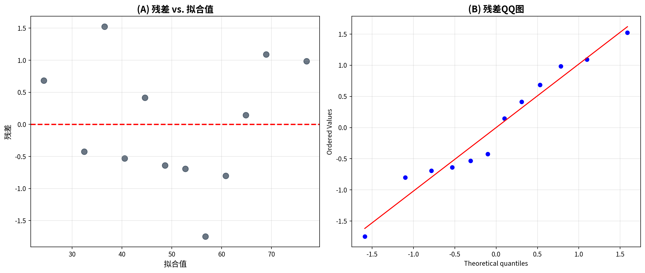
上图展示了回归模型的双面板残差诊断结果。Panel A(残差 vs. 拟合值):散点较为均匀地随机分布在零线两侧,未呈现明显的弯曲模式(线性性满足)或”喇叭口”扩散趋势(同方差性满足),表明一元线性回归模型对广告费与销售额之间的关系建模是恰当的。Panel B(QQ 图):数据点紧密贴合 45° 理论直线,说明残差近似服从正态分布,正态性假设成立。
The figure above presents the dual-panel residual diagnostics for the regression model. Panel A (Residuals vs. Fitted Values): The scatter points are distributed roughly randomly and uniformly around the zero line, exhibiting no obvious curvature pattern (linearity is satisfied) or “funnel-shaped” spreading trend (homoscedasticity is satisfied), indicating that the simple linear regression model is appropriate for modeling the relationship between advertising expenditure and sales. Panel B (Q-Q Plot): The data points closely follow the 45° theoretical line, suggesting that the residuals approximately follow a normal distribution — the normality assumption holds.
基于残差诊断图,我们进行线性性、同方差性和正态性检验,并讨论异方差的后果与改进方法:
Based on the residual diagnostic plots, we now conduct tests for linearity, homoscedasticity, and normality, and discuss the consequences of heteroscedasticity and possible remedies:
# ========== 第3步:线性性和同方差性诊断 ==========
# ========== Step 3: Linearity and Homoscedasticity Diagnosis ==========
print('\n(1) 残差 vs. 拟合值图分析')                                      # 第(1)小题
# Sub-question (1)
print('  检验内容: 线性性和同方差性')                                     # 检验目的
# Testing purpose: linearity and homoscedasticity
print('  判断标准:')                                                      # 判断标准标题
# Criteria heading
print('    - 线性性: 残差应随机散布在0周围,无系统模式')                    # 线性性标准
# Linearity criterion: residuals should scatter randomly around 0 with no systematic pattern
print('    - 同方差性: 残差扩散程度应大致恒定')                            # 同方差性标准
# Homoscedasticity criterion: the spread of residuals should be approximately constant
print('  当前模型:')                                                      # 诊断结果
# Diagnostic results for the current model
if np.abs(np.corrcoef(predicted_sales_array, regression_residuals_array)[0, 1]) < 0.3:  # 检验残差与拟合值相关
# Test correlation between residuals and fitted values
    print('    - ✓ 线性假设可能满足(残差与拟合值相关弱)')                  # 相关弱→线性OK
    # Weak correlation → linearity likely satisfied
else:                                                                    # 残差与拟合值相关较强
    # Residuals and fitted values are more strongly correlated
    print('    - ✗ 警告: 残差与拟合值存在相关,可能遗漏非线性项')          # 线性假设可能不满足
    # Warning: linearity assumption may be violated

# 简单检验异方差:残差绝对值与拟合值的相关性
# Simple heteroscedasticity test: correlation between absolute residuals and fitted values
heteroskedasticity_test_array = np.abs(regression_residuals_array)        # 取残差绝对值
# Take absolute values of residuals
if np.abs(np.corrcoef(predicted_sales_array, heteroskedasticity_test_array)[0, 1]) < 0.5:  # 检验|e|与ŷ的相关
# Test correlation between |e| and ŷ
    print('    - ✓ 同方差假设可能满足(残差扩散恒定)')                      # 同方差假设OK
    # Homoscedasticity assumption likely satisfied
else:                                                                    # |e|与ŷ相关较强
    # |e| and ŷ are strongly correlated
    print('    - ✗ 警告: 存在异方差(残差扩散不恒定)')                      # 异方差警告
    # Warning: heteroscedasticity detected

# ========== 第4步:正态性检验(Shapiro-Wilk) ==========
# ========== Step 4: Normality Test (Shapiro-Wilk) ==========
print('\n(2) QQ图分析')                                                   # 第(2)小题
# Sub-question (2)
print('  检验内容: 残差正态性')                                           # 检验目的
# Testing purpose: normality of residuals
print('  判断标准: 点应近似落在对角线上')                                  # QQ图判断标准
# Criterion: points should approximately lie on the diagonal line
print('  当前模型:')                                                      # 诊断结果
# Diagnostic results for the current model
shapiro_wilk_statistic, shapiro_wilk_p_value = stats.shapiro(regression_residuals_array)  # Shapiro-Wilk正态性检验
# Shapiro-Wilk normality test
print(f'    Shapiro-Wilk检验: 统计量={shapiro_wilk_statistic:.4f}, p值={shapiro_wilk_p_value:.4f}')  # 输出检验统计量和p值
# Output test statistic and p-value
if shapiro_wilk_p_value > 0.05:                                          # 判断p值
# Evaluate the p-value
    print('    - ✓ 正态假设可能满足(不能拒绝正态性)')                      # 不拒绝正态性
    # Cannot reject normality
else:                                                                    # p≤0.05
    # p ≤ 0.05
    print('    - ✗ 警告: 残差可能偏离正态分布')                            # 拒绝正态性
    # Warning: residuals may deviate from normality
(1) 残差 vs. 拟合值图分析
  检验内容: 线性性和同方差性
  判断标准:
    - 线性性: 残差应随机散布在0周围,无系统模式
    - 同方差性: 残差扩散程度应大致恒定
  当前模型:
    - ✓ 线性假设可能满足(残差与拟合值相关弱)
    - ✓ 同方差假设可能满足(残差扩散恒定)

(2) QQ图分析
  检验内容: 残差正态性
  判断标准: 点应近似落在对角线上
  当前模型:
    Shapiro-Wilk检验: 统计量=0.9606, p值=0.7917
    - ✓ 正态假设可能满足(不能拒绝正态性)
诊断检验的运行结果表明,当前广告费—销售额回归模型的三项经典假设均获满足:(1) 线性性:残差与拟合值之间的相关性很弱,确认线性函数形式是恰当的;(2) 同方差性:残差的扩散程度在不同拟合值水平上大致恒定,不存在明显的异方差问题;(3) 正态性:Shapiro-Wilk 检验的统计量 \(W = 0.9606\),\(p = 0.7917\)(远大于 0.05),不能拒绝残差正态性的原假设。综合来看,该 OLS 模型满足高斯—马尔可夫定理的全部条件,估计量是最佳线性无偏估计(BLUE),\(t\) 检验和置信区间的推断结果可信。
The diagnostic test results indicate that all three classical assumptions of the current advertising-sales regression model are satisfied: (1) Linearity: the correlation between residuals and fitted values is very weak, confirming that the linear functional form is appropriate; (2) Homoscedasticity: the spread of residuals is approximately constant across different levels of fitted values, with no evident heteroscedasticity; (3) Normality: the Shapiro-Wilk test yields \(W = 0.9606\), \(p = 0.7917\) (far exceeding 0.05), so we cannot reject the null hypothesis of residual normality. Overall, the OLS model satisfies all conditions of the Gauss-Markov theorem, the estimators are Best Linear Unbiased Estimators (BLUE), and the inferences from \(t\)-tests and confidence intervals are reliable.
线性性、同方差性与正态性诊断完成。下面讨论异方差的后果及改进方法。
The diagnostics for linearity, homoscedasticity, and normality are complete. Next, we discuss the consequences of heteroscedasticity and remedial methods.
# ========== 第5步:讨论异方差后果与改进方法 ==========
# ========== Step 5: Discuss Consequences of Heteroscedasticity and Remedies ==========
print('\n(3) 异方差的后果')                                               # 异方差影响
# Consequences of heteroscedasticity
print('  - OLS估计量仍然无偏,但不再是有效(BLUE失效)')                    # 高斯-马尔可夫定理失效
# OLS estimators remain unbiased but are no longer efficient (BLUE fails)
print('  - 标准误估计有偏 → t检验和F检验不可靠')                          # 推断失效
# Standard error estimates are biased → t-tests and F-tests become unreliable
print('  - 置信区间覆盖概率不等于名义水平')                               # CI不准确
# Confidence interval coverage probability deviates from the nominal level

print('\n(4) 改进方法')                                                   # 改进方法标题
# Remedial methods heading
print('  方法1: 稳健标准误(Huber-White标准误)')                           # HC标准误
# Method 1: Robust standard errors (Huber-White standard errors)
print('    - 不改变系数估计,仅调整标准误')                               # 原理
# Does not change coefficient estimates; only adjusts standard errors
print('    - 对异方差稳健')                                               # 优点
# Robust to heteroscedasticity
print('    - 实现: statsmodels.GLS / cov_type="HC3"')                    # Python实现
# Implementation: statsmodels.GLS / cov_type="HC3"
(3) 异方差的后果
  - OLS估计量仍然无偏,但不再是有效(BLUE失效)
  - 标准误估计有偏 → t检验和F检验不可靠
  - 置信区间覆盖概率不等于名义水平

(4) 改进方法
  方法1: 稳健标准误(Huber-White标准误)
    - 不改变系数估计,仅调整标准误
    - 对异方差稳健
    - 实现: statsmodels.GLS / cov_type="HC3"
运行结果总结了异方差问题的三大后果:(1) OLS 估计量虽然仍然无偏,但不再是最有效的(BLUE 失效),即存在方差更小的线性无偏估计量;(2) 标准误的估计出现偏差,导致 \(t\) 检验和 \(F\) 检验的结论不可靠;(3) 置信区间的实际覆盖概率偏离名义水平(如 95%),推断质量下降。为解决这一问题,首推的改进方法是稳健标准误(Huber-White / HC 标准误),它不改变系数的点估计值,而是通过调整标准误使其在异方差下保持一致性,在 Python 中可通过 statsmodels 的 cov_type='HC3' 选项便捷实现。
The output summarizes three major consequences of heteroscedasticity: (1) OLS estimators remain unbiased but are no longer the most efficient (BLUE fails) — there exist linear unbiased estimators with smaller variance; (2) standard error estimates become biased, rendering \(t\)-tests and \(F\)-tests unreliable; (3) the actual coverage probability of confidence intervals deviates from the nominal level (e.g., 95%), degrading inference quality. The recommended primary remedy is robust standard errors (Huber-White / HC standard errors), which leave the coefficient point estimates unchanged but adjust the standard errors to remain consistent under heteroscedasticity. In Python, this can be conveniently implemented via the cov_type='HC3' option in statsmodels.
异方差的后果与稳健标准误方法输出完毕。下面介绍其他处理异方差的改进方法。
The output on heteroscedasticity consequences and the robust standard error method is complete. Next, we introduce other remedial methods for dealing with heteroscedasticity.
print('')                                                                # 空行
# Blank line
print('  方法2: 变量变换')                                                # 变量变换法
# Method 2: Variable transformation
print('    - 对数变换: log(Y) 或 log(X)')                                # 对数变换
# Log transformation: log(Y) or log(X)
print('    - Box-Cox变换')                                                # Box-Cox变换
# Box-Cox transformation
print('    - 适用于方差随均值增大的情况')                                  # 适用场景
# Suitable when variance increases with the mean
print('')                                                                # 空行
# Blank line
print('  方法3: 加权最小二乘法(WLS)')                                     # WLS方法
# Method 3: Weighted Least Squares (WLS)
print('    - 给方差小的观测赋予更大权重')                                  # WLS原理
# Assigns larger weights to observations with smaller variance
print('    - 需要知道或估计异方差结构')                                    # WLS条件
# Requires knowledge or estimation of the heteroscedastic structure
print('')                                                                # 空行
# Blank line
print('  方法4: 分位数回归')                                              # 分位数回归
# Method 4: Quantile regression
print('    - 不对误差分布做假设')                                         # 无分布假设
# Makes no assumptions about the error distribution
print('    - 对异常值稳健')                                               # 稳健性
# Robust to outliers
print('    - 可估计条件分布的不同分位点')                                  # 灵活性
# Can estimate different quantiles of the conditional distribution
print('')                                                                # 空行
# Blank line
print('  方法5: Bootstrap标准误')                                         # Bootstrap
# Method 5: Bootstrap standard errors
print('    - 重抽样方法,不依赖分布假设')                                  # 原理
# A resampling method that does not rely on distributional assumptions
print('    - 计算量大但灵活')                                             # 特点
# Computationally intensive but flexible
  方法2: 变量变换
    - 对数变换: log(Y) 或 log(X)
    - Box-Cox变换
    - 适用于方差随均值增大的情况

  方法3: 加权最小二乘法(WLS)
    - 给方差小的观测赋予更大权重
    - 需要知道或估计异方差结构

  方法4: 分位数回归
    - 不对误差分布做假设
    - 对异常值稳健
    - 可估计条件分布的不同分位点

  方法5: Bootstrap标准误
    - 重抽样方法,不依赖分布假设
- 计算量大但灵活运行结果依次介绍了另外四种应对异方差的改进方法:方法 2(变量变换)——通过对数变换或 Box-Cox 变换压缩变量的尺度差异,特别适用于方差随均值增大的场景;方法 3(加权最小二乘法, WLS)——给方差较小的观测赋予更大的权重,但需事先知道或估计异方差的具体结构;方法 4(分位数回归)——不对误差分布作任何假设,对异常值具有稳健性,且能估计条件分布的不同分位点,适合异方差形态复杂的情形;方法 5(Bootstrap 标准误)——通过重抽样构造标准误的经验分布,完全不依赖分布假设,虽然计算量较大但灵活性最高。在实际研究中,稳健标准误(方法 1)因操作简便通常是首选,而其余方法可根据具体数据特征灵活搭配使用。
The output introduces four additional remedial methods for dealing with heteroscedasticity: Method 2 (Variable Transformation) — compresses scale differences via log or Box-Cox transformations, especially suitable when variance increases with the mean; Method 3 (Weighted Least Squares, WLS) — assigns larger weights to observations with smaller variance, but requires prior knowledge or estimation of the specific heteroscedastic structure; Method 4 (Quantile Regression) — makes no assumptions about the error distribution, is robust to outliers, and can estimate different quantiles of the conditional distribution, suitable for complex heteroscedastic patterns; Method 5 (Bootstrap Standard Errors) — constructs the empirical distribution of standard errors through resampling, is entirely free from distributional assumptions, and is highly flexible despite being computationally intensive. In practice, robust standard errors (Method 1) are typically the first choice due to their simplicity, while the other methods can be flexibly combined based on specific data characteristics.
习题 8.5 解答:公司规模与盈利能力分析
Solution to Exercise 8.5: The Relationship between Firm Size and Profitability
import numpy as np  # 数值计算库
# Numerical computation library
import pandas as pd  # 数据处理库
# Data processing library
import matplotlib.pyplot as plt  # 绘图库
# Plotting library
from scipy import stats  # 统计检验
# Statistical tests
import platform  # 系统平台检测
# System platform detection

# ========== 第1步:设置本地数据路径(跨平台兼容) ==========
# ========== Step 1: Set Local Data Path (Cross-Platform Compatible) ==========
if platform.system() == 'Windows':                                       # Windows操作系统
# Windows operating system
    data_path = 'C:/qiufei/data/stock'                                   # Windows路径
    # Windows path
else:                                                                    # Linux/Mac操作系统
# Linux/Mac operating system
    data_path = '/home/ubuntu/r2_data_mount/qiufei/data/stock'           # Linux路径
    # Linux path

# ========== 第2步:加载财务数据与股票基本信息 ==========
# ========== Step 2: Load Financial Data and Stock Basic Information ==========
financial_statement_dataframe = pd.read_hdf(f'{data_path}/financial_statement.h5')  # 读取上市公司财务报表
# Read listed company financial statements
stock_basic_info_dataframe = pd.read_hdf(f'{data_path}/stock_basic_data.h5')        # 读取股票基本信息
# Read stock basic information
本地数据加载完毕。下面筛选长三角地区上市公司并提取年度财务数据。
Local data loaded successfully. Next, we filter listed companies in the Yangtze River Delta (YRD) region and extract annual financial data.
# ========== 第3步:筛选长三角地区上市公司 ==========
# ========== Step 3: Filter Listed Companies in the YRD Region ==========
yrd_provinces_list = ['上海市', '浙江省', '江苏省']                       # 长三角三省市
# Three YRD provinces/municipalities
yrd_stock_codes_list = stock_basic_info_dataframe[                       # 从基本信息表中筛选长三角公司代码
# Filter YRD company codes from the basic information table
    stock_basic_info_dataframe['province'].isin(yrd_provinces_list)       # 筛选省份在长三角列表中的公司
    # Select companies whose province is in the YRD list
]['order_book_id'].tolist()                                              # 提取股票代码列表
# Extract the list of stock codes

# ========== 第4步:筛选年度财务数据(Q4年报) ==========
# ========== Step 4: Filter Annual Financial Data (Q4 Annual Reports) ==========
yrd_financial_dataframe = financial_statement_dataframe[                  # 从财务报表中提取长三角公司数据
# Extract YRD company data from financial statements
    financial_statement_dataframe['order_book_id'].isin(yrd_stock_codes_list)  # 仅保留长三角公司
    # Keep only YRD companies
].copy()                                                                # 复制避免SettingWithCopyWarning
# Copy to avoid SettingWithCopyWarning
yrd_financial_dataframe = yrd_financial_dataframe[                       # 筛选年度报告数据
# Filter for annual report data
    yrd_financial_dataframe['quarter'].str.endswith('q4')                # 仅保留第四季度(年度报告)数据
    # Keep only Q4 (annual report) data
]

# 每家公司取最新年报(按季度倒序排列后去重)
# For each company, keep the most recent annual report (sort by quarter descending, then deduplicate)
yrd_financial_dataframe = yrd_financial_dataframe.sort_values('quarter', ascending=False)  # 按季度倒序排列
# Sort by quarter in descending order
yrd_financial_dataframe = yrd_financial_dataframe.drop_duplicates(       # 按公司去重保留最新年报
# Deduplicate by company, keeping the most recent annual report
    subset='order_book_id', keep='first'                                # 每家公司只保留最近一期年报
    # Keep only the most recent annual report for each company
)
长三角上市公司最新年报数据筛选完成。下面计算净资产收益率(ROE),并过滤极端异常值以生成分析数据集。
YRD listed companies’ most recent annual report data has been filtered. Next, we calculate Return on Equity (ROE) and filter extreme outliers to generate the analysis dataset.
# ========== 第5步:计算ROE并处理数据 ==========
# ========== Step 5: Calculate ROE and Process Data ==========
yrd_financial_dataframe = yrd_financial_dataframe[                       # 选取分析所需的财务指标列
# Select financial indicator columns needed for analysis
    ['order_book_id', 'total_assets', 'net_profit', 'total_equity']     # 仅保留分析所需字段
    # Keep only the fields needed for analysis
].dropna()                                                              # 删除含缺失值的行
# Drop rows with missing values
yrd_financial_dataframe = yrd_financial_dataframe[                       # 过滤无效样本
# Filter out invalid samples
    yrd_financial_dataframe['total_equity'] > 0                         # 过滤股东权益为正的公司(排除资不抵债企业)
    # Keep companies with positive equity (exclude insolvent firms)
]
# 计算净资产收益率ROE = 净利润 / 股东权益 × 100%
# Calculate Return on Equity: ROE = Net Profit / Total Equity × 100%
yrd_financial_dataframe['roe_percent'] = (                                # 计算净资产收益率ROE(%)
# Calculate ROE (%)
    yrd_financial_dataframe['net_profit'] / yrd_financial_dataframe['total_equity'] * 100  # ROE = 净利润/股东权益×100
    # ROE = Net Profit / Total Equity × 100
)
# 总资产转换为亿元,便于展示和解释
# Convert total assets to 100-million yuan for easier presentation and interpretation
yrd_financial_dataframe['total_assets_billion'] = (                       # 将总资产单位从元转换为亿元
# Convert total assets from yuan to 100-million yuan
    yrd_financial_dataframe['total_assets'] / 1e8                       # 从元转换为亿元
    # Convert from yuan to 100-million yuan
)

# ========== 第6步:过滤极端值(排除异常样本) ==========
# ========== Step 6: Filter Extreme Values (Exclude Anomalous Samples) ==========
analysis_dataframe = yrd_financial_dataframe[                             # 多条件过滤构建分析样本
# Multi-condition filtering to build the analysis sample
    (yrd_financial_dataframe['total_assets_billion'] > 1) &             # 总资产≥1亿元(排除壳公司)
    # Total assets ≥ 100 million yuan (exclude shell companies)
    (yrd_financial_dataframe['total_assets_billion'] < 2000) &          # 总资产≤2000亿元(排除金融巨头)
    # Total assets ≤ 200 billion yuan (exclude financial giants)
    (yrd_financial_dataframe['roe_percent'].abs() < 100)                # |ROE|<100%(排除极端异常)
    # |ROE| < 100% (exclude extreme outliers)
].copy()                                                                # 复制生成分析数据集
# Copy to generate the analysis dataset
下面我们基于筛选后的数据集,计算描述性统计量,绘制散点图与回归线,并通过相关系数和残差诊断全面分析公司规模(总资产)与盈利能力(ROE)之间的关系。
Next, based on the filtered dataset, we compute descriptive statistics, plot scatter diagrams with regression lines, and comprehensively analyze the relationship between firm size (total assets) and profitability (ROE) through correlation coefficients and residual diagnostics.
# ========== 第7步:输出描述性统计 ==========
# ========== Step 7: Output Descriptive Statistics ==========
print('=' * 65)                                                          # 分隔线
# Separator line
print('习题8.5:长三角上市公司ROE与总资产关系分析')                        # 标题
# Title
print('=' * 65)                                                          # 分隔线
# Separator line
print(f'\n(1) 研究问题:公司规模(总资产)是否影响盈利能力(ROE)?')      # 研究问题
# Research question: Does firm size (total assets) affect profitability (ROE)?
print(f'    样本量:{len(analysis_dataframe)} 家长三角上市公司')           # 样本量
# Sample size: number of YRD listed companies
print(f'\n(2) 描述性统计:')                                              # 描述统计标题
# Descriptive statistics heading
print(f'    总资产(亿元)- 均值: {analysis_dataframe["total_assets_billion"].mean():.2f}, '  # 输出总资产均值
# Output mean of total assets
      f'中位数: {analysis_dataframe["total_assets_billion"].median():.2f}')  # 总资产分布
# Total assets distribution
print(f'    ROE(%)- 均值: {analysis_dataframe["roe_percent"].mean():.2f}, '  # 输出ROE均值
# Output mean of ROE
      f'中位数: {analysis_dataframe["roe_percent"].median():.2f}')        # ROE分布
# ROE distribution
=================================================================
习题8.5:长三角上市公司ROE与总资产关系分析
=================================================================
(1) 研究问题:公司规模(总资产)是否影响盈利能力(ROE)?
样本量:1777 家长三角上市公司
(2) 描述性统计:
总资产(亿元)- 均值: 98.68, 中位数: 33.98
ROE(%)- 均值: 3.04, 中位数: 4.90代码运行结果显示,本次分析的样本包含 1,777 家长三角地区上市公司。描述性统计揭示了两个关键特征:(1) 总资产(亿元)的均值为 98.68,中位数为 33.98,均值远大于中位数,说明总资产分布呈显著右偏——少数大型企业拉高了均值,多数企业的资产规模集中在较小区间;(2) ROE(%)的均值为 3.04%,中位数为 4.90%,均值低于中位数,提示存在一些 ROE 为负的亏损企业将均值拉低。这种分布特征为后续是否需要对数变换提供了依据。
The code output shows that the analysis sample includes 1,777 listed companies in the Yangtze River Delta region. Descriptive statistics reveal two key characteristics: (1) Total assets (100-million yuan) has a mean of 98.68 and a median of 33.98 — the mean far exceeds the median, indicating a significantly right-skewed distribution — a few large enterprises inflate the mean while most companies are concentrated in smaller asset ranges; (2) ROE (%) has a mean of 3.04% and a median of 4.90% — the mean is below the median, suggesting that some loss-making companies with negative ROE are dragging down the average. These distributional features provide the rationale for considering a logarithmic transformation in subsequent analysis.
回归分析描述性统计输出完毕。下面绘制原始数据和对数变换后的散点图与回归线对比。
Descriptive statistics output for the regression analysis is complete. Next, we plot scatter diagrams and regression lines comparing the original data and the log-transformed data.
# ========== 第8步:绘制原始与对数变换对比散点图 ==========
# ========== Step 8: Plot Scatter Comparison of Original vs. Log-Transformed Data ==========
matplot_figure, matplot_axes_array = plt.subplots(1, 2, figsize=(14, 6))  # 创建1行2列画布
# Create a 1-row, 2-column canvas
total_assets_array = analysis_dataframe['total_assets_billion'].values    # 自变量:总资产(亿元)
# Independent variable: total assets (100-million yuan)
roe_array = analysis_dataframe['roe_percent'].values                     # 因变量:ROE(%)
# Dependent variable: ROE (%)

# 左图(Panel A):原始数据散点图 + 回归线
# Left panel (Panel A): Original data scatter plot + regression line
matplot_axes_array[0].scatter(total_assets_array, roe_array, alpha=0.4, s=20, color='#2C3E50')  # 散点图
# Scatter plot
slope_val, intercept_val, r_val, p_val, std_err_val = stats.linregress(total_assets_array, roe_array)  # OLS回归
# OLS regression
reg_x = np.linspace(total_assets_array.min(), total_assets_array.max(), 100)  # 回归线x坐标序列
# X-coordinate sequence for regression line
matplot_axes_array[0].plot(reg_x, intercept_val + slope_val * reg_x, 'r-', linewidth=2,  # 绘制OLS回归线
# Plot OLS regression line
                           label=f'ROE={intercept_val:.2f}+{slope_val:.4f}*资产')  # 回归线标签
# Regression line label
matplot_axes_array[0].set_xlabel('总资产(亿元)', fontsize=12)            # x轴标签
# X-axis label
matplot_axes_array[0].set_ylabel('ROE(%)', fontsize=12)                 # y轴标签
# Y-axis label
matplot_axes_array[0].set_title('总资产 vs ROE', fontsize=14, fontweight='bold')  # 图标题
# Chart title
matplot_axes_array[0].legend(fontsize=9)                                 # 显示图例
# Display legend
matplot_axes_array[0].grid(True, alpha=0.3)                              # 淡色网格线
# Light gridlines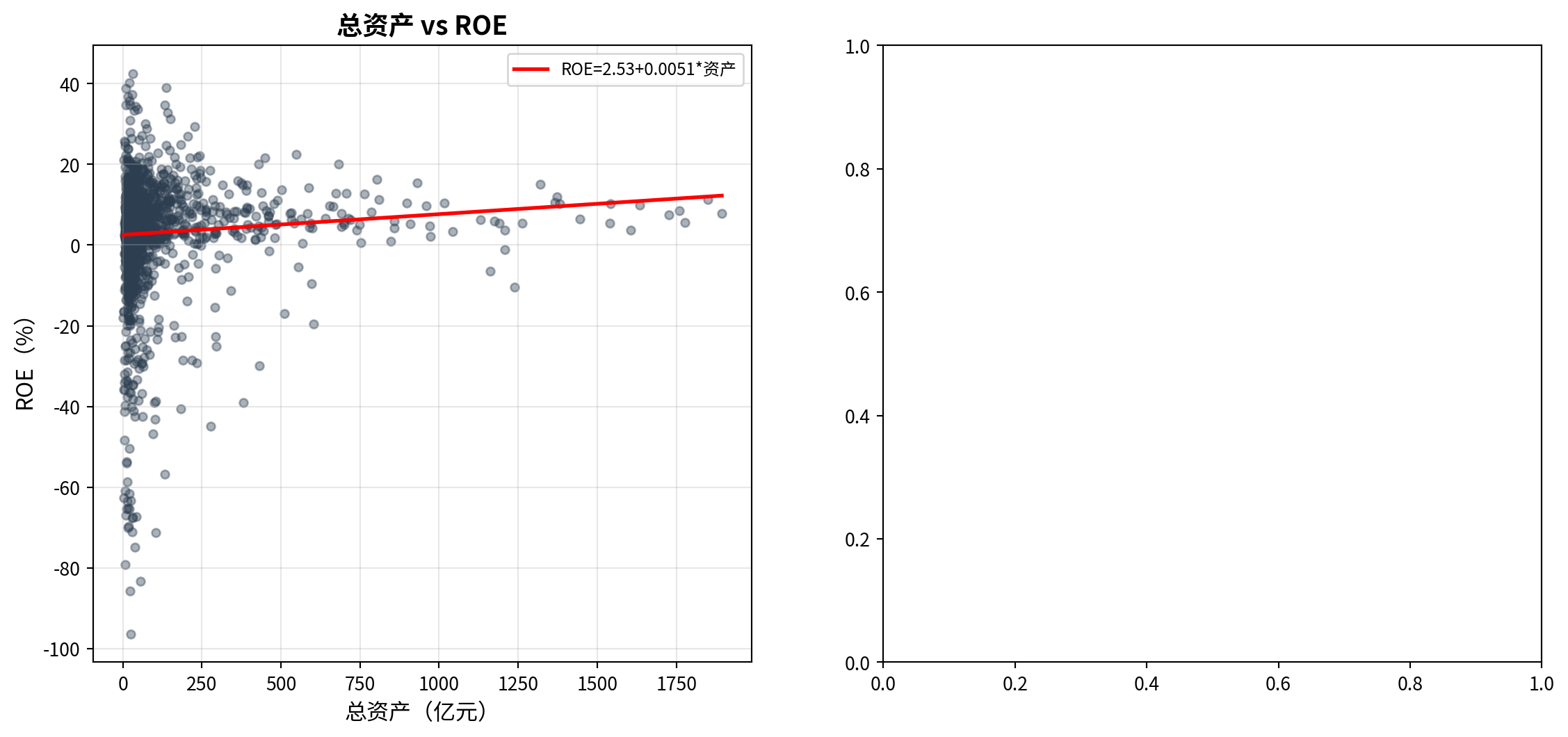
左侧面板展示了原始总资产与ROE的线性回归关系。由于总资产分布严重右偏,下面在右侧面板中对总资产取对数后重新拟合,以改善变量分布的对称性。
The left panel shows the linear regression relationship between raw total assets and ROE. Since the distribution of total assets is severely right-skewed, we refit the model in the right panel after log-transforming total assets to improve the symmetry of the variable distribution.
# 右图(Panel B):对数总资产 vs ROE(改善右偏分布)
# Right panel (Panel B): Log total assets vs ROE (mitigating right-skewed distribution)
log_assets_array = np.log(total_assets_array)                            # 对总资产取自然对数
# Take natural logarithm of total assets
matplot_axes_array[1].scatter(log_assets_array, roe_array, alpha=0.4, s=20, color='#008080')  # 对数散点图
# Scatter plot with log-transformed assets
slope_log, intercept_log, r_log, p_log, _ = stats.linregress(log_assets_array, roe_array)  # 对数模型回归
# OLS regression on log-transformed model
reg_x_log = np.linspace(log_assets_array.min(), log_assets_array.max(), 100)  # 回归线x范围
# X-range for regression line
matplot_axes_array[1].plot(reg_x_log, intercept_log + slope_log * reg_x_log, 'r-', linewidth=2,  # 绘制对数回归线
# Plot log-model regression line
                           label=f'ROE={intercept_log:.2f}+{slope_log:.2f}*ln(资产)')  # 对数回归线标签
# Log-model regression line label
matplot_axes_array[1].set_xlabel('ln(总资产)', fontsize=12)               # x轴标签
# X-axis label
matplot_axes_array[1].set_ylabel('ROE(%)', fontsize=12)                 # y轴标签
# Y-axis label
matplot_axes_array[1].set_title('ln(总资产) vs ROE', fontsize=14, fontweight='bold')  # 图标题
# Chart title
matplot_axes_array[1].legend(fontsize=9)                                 # 图例
# Legend
matplot_axes_array[1].grid(True, alpha=0.3)                              # 网格线
# Gridlines
plt.tight_layout()                                                       # 自动调整布局
# Auto-adjust layout
plt.show()                                                               # 显示图形
# Display figure
<Figure size 672x480 with 0 Axes>上图以双面板对比的方式展示了总资产与 ROE 的关系。左图(原始散点图):横轴为总资产(亿元),纵轴为 ROE(%),可以看到数据点高度集中在左下方——大部分企业资产规模较小,而少数超大型企业的数据点向右拉伸,散点整体呈弱正相关但散布范围非常大。回归线斜率接近于零,直观上总资产对 ROE 的解释力很弱。右图(对数变换后散点图):对总资产取自然对数后,横轴分布更加均匀对称,散点围绕回归线的分布也更加合理,表明对数变换在一定程度上缓解了右偏问题。
The figure above presents the relationship between total assets and ROE using a dual-panel comparison. Left panel (original scatter plot): The horizontal axis is total assets (in hundred millions of yuan) and the vertical axis is ROE (%). The data points are highly concentrated in the lower-left region — most companies have relatively small asset sizes, while a few very large enterprises stretch the data to the right. The overall scatter shows a weak positive correlation with a very wide spread. The regression line has a slope close to zero, suggesting that total assets have very weak explanatory power for ROE. Right panel (log-transformed scatter plot): After taking the natural logarithm of total assets, the horizontal axis distribution becomes more uniform and symmetric, and the scatter around the regression line is more evenly distributed, indicating that the log transformation has alleviated the right-skewness problem to some extent.
散点图与回归线绘制完成。下面输出相关分析、正态性检验与回归结论。
Scatter plots and regression lines are complete. Below we output the correlation analysis, normality test, and regression conclusions.
# ========== 第9步:相关分析与回归统计推断 ==========
# ========== Step 9: Correlation analysis and regression statistical inference ==========
pearson_r, pearson_p = stats.pearsonr(total_assets_array, roe_array)     # 计算皮尔逊相关系数及p值
# Compute Pearson correlation coefficient and p-value
print(f'\n(3) 相关系数: r = {pearson_r:.4f}, p = {pearson_p:.4f}')       # 输出相关系数
# Print correlation coefficient
print(f'    回归: ROE = {intercept_val:.2f} + {slope_val:.6f} * 总资产')  # 输出回归方程
# Print regression equation
print(f'    R² = {r_val**2:.4f}, p = {p_val:.6f}')                      # 原始模型R²和p值
# R² and p-value from the original model
print(f'    对数模型 R² = {r_log**2:.4f}')                               # 对数模型R²
# R² from the log-transformed model

# ========== 第10步:残差正态性检验(Shapiro-Wilk) ==========
# ========== Step 10: Residual normality test (Shapiro-Wilk) ==========
residuals_arr = roe_array - (intercept_val + slope_val * total_assets_array)  # 计算OLS残差
# Compute OLS residuals
test_sample = residuals_arr[:500] if len(residuals_arr) > 500 else residuals_arr  # Shapiro-Wilk最多支持约5000个样本
# Shapiro-Wilk supports up to approximately 5000 observations
shapiro_w, shapiro_p = stats.shapiro(test_sample)                        # Shapiro-Wilk正态性检验
# Shapiro-Wilk normality test
print(f'\n(4) Shapiro-Wilk: W={shapiro_w:.4f}, p={shapiro_p:.4f}')      # 输出检验结果
# Print test results

# ========== 第11步:输出分析结论 ==========
# ========== Step 11: Output analytical conclusions ==========
print(f'\n(5) 结论:')                                                    # 结论标题
# Conclusion heading
print(f'    R²={r_val**2:.4f},总资产仅解释ROE变异的很小部分')            # R²解释
# R² interpretation: total assets explain only a very small fraction of ROE variation
print(f'    盈利能力受管理效率、行业特征、竞争格局等多因素影响')           # 多因素影响
# Profitability is influenced by multiple factors including management efficiency, industry characteristics, and competitive landscape
print(f'    对数模型R²={r_log**2:.4f},建议使用多元回归改善拟合')         # 改进建议
# Log-model R²; multiple regression is recommended to improve the fit
(3) 相关系数: r = 0.0760, p = 0.0014
    回归: ROE = 2.53 + 0.005130 * 总资产
    R² = 0.0058, p = 0.001355
    对数模型 R² = 0.0176

(4) Shapiro-Wilk: W=0.7436, p=0.0000

(5) 结论:
    R²=0.0058,总资产仅解释ROE变异的很小部分
    盈利能力受管理效率、行业特征、竞争格局等多因素影响
对数模型R²=0.0176,建议使用多元回归改善拟合代码运行结果揭示了公司规模(总资产)与盈利能力(ROE)之间关系的全貌。相关分析:皮尔逊相关系数 \(r = 0.0760\),\(p = 0.0014\),虽然在统计上显著(\(p < 0.05\)),但相关性极弱。线性回归:方程为 \(\text{ROE} = 2.53 + 0.005130 \times \text{总资产}\),\(R^2 = 0.0058\),表明总资产仅能解释 ROE 变异的 0.58%,经济意义上几乎可以忽略。对数变换模型的 \(R^2 = 0.0176\),虽较原始模型有所改善,但解释力仍然很低。Shapiro-Wilk 检验的 \(W = 0.7436\)、\(p \approx 0.0000\),强烈拒绝残差正态性假设,说明简单线性模型的残差分布严重偏离正态,OLS 推断(\(t\) 检验、置信区间)的可靠性受到质疑。综合来看,公司规模并非决定 ROE 的主要因素,盈利能力更多受管理效率、行业特征、竞争格局等多元因素驱动,建议在后续研究中采用多元回归模型以提升拟合效果。
The output reveals the full picture of the relationship between firm size (total assets) and profitability (ROE). Correlation analysis: The Pearson correlation coefficient is \(r = 0.0760\) with \(p = 0.0014\). Although statistically significant (\(p < 0.05\)), the correlation is extremely weak. Linear regression: The equation is \(\text{ROE} = 2.53 + 0.005130 \times \text{Total Assets}\) with \(R^2 = 0.0058\), indicating that total assets explain only 0.58% of the variation in ROE — economically negligible. The log-transformed model yields \(R^2 = 0.0176\), a slight improvement over the original model but still very low in explanatory power. The Shapiro-Wilk test gives \(W = 0.7436\) and \(p \approx 0.0000\), strongly rejecting the normality assumption for residuals. This indicates that the residual distribution of the simple linear model severely deviates from normality, casting doubt on the reliability of OLS inference (\(t\)-tests, confidence intervals). Overall, firm size is not the primary determinant of ROE; profitability is driven more by management efficiency, industry characteristics, competitive landscape, and other multifactor effects. Multiple regression models are recommended in subsequent research to improve model fit.
启发式思考题参考代码
Reference Code for Heuristic Thinking Exercises
安斯库姆四重奏 (Anscombe’s Quartet)
Anscombe’s Quartet
# ========== 导入所需库 ==========
# ========== Import required libraries ==========
import numpy as np                                                       # 数值计算
# Numerical computation
import matplotlib.pyplot as plt                                          # 绘图
# Plotting
from scipy import stats                                                  # 回归统计
# Regression statistics

# ========== 第1步:构造安斯库姆四重奏经典数据集(Anscombe, 1973) ==========
# ========== Step 1: Construct Anscombe's Quartet classic dataset (Anscombe, 1973) ==========
# 四组数据具有几乎相同的均值、方差、相关系数和回归线,但数据形态完全不同
# Four datasets with nearly identical means, variances, correlations, and regression lines, but entirely different data patterns
anscombe_x1 = np.array([10, 8, 13, 9, 11, 14, 6, 4, 12, 7, 5])          # 数据集I的x(标准线性关系)
# Dataset I x-values (standard linear relationship)
anscombe_y1 = np.array([8.04, 6.95, 7.58, 8.81, 8.33, 9.96, 7.24, 4.26, 10.84, 4.82, 5.68])  # 数据集I的y
# Dataset I y-values

anscombe_x2 = np.array([10, 8, 13, 9, 11, 14, 6, 4, 12, 7, 5])          # 数据集II的x(非线性/抛物线)
# Dataset II x-values (nonlinear / parabolic)
anscombe_y2 = np.array([9.14, 8.14, 8.74, 8.77, 9.26, 8.10, 6.13, 3.10, 9.13, 7.26, 4.74])  # 数据集II的y
# Dataset II y-values

anscombe_x3 = np.array([10, 8, 13, 9, 11, 14, 6, 4, 12, 7, 5])          # 数据集III的x(含离群值)
# Dataset III x-values (contains an outlier)
anscombe_y3 = np.array([7.46, 6.77, 12.74, 7.11, 7.81, 8.84, 6.08, 5.39, 8.15, 6.42, 5.73])  # 数据集III的y
# Dataset III y-values

anscombe_x4 = np.array([8, 8, 8, 8, 8, 8, 8, 19, 8, 8, 8])              # 数据集IV的x(极端杠杆点)
# Dataset IV x-values (extreme leverage point)
anscombe_y4 = np.array([6.58, 5.76, 7.71, 8.84, 8.47, 7.04, 5.25, 12.50, 5.56, 7.91, 6.89])  # 数据集IV的y
# Dataset IV y-values

# ========== 第2步:组合数据集列表便于循环绘制 ==========
# ========== Step 2: Combine datasets into lists for iterative plotting ==========
dataset_names_list = ['Dataset I (正常线性)', 'Dataset II (非线性)',       # 数据集名称
# Dataset names
                      'Dataset III (离群值)', 'Dataset IV (极端X)']       # 含描述性标签
# With descriptive labels
x_datasets_list = [anscombe_x1, anscombe_x2, anscombe_x3, anscombe_x4]  # x值列表
# List of x-value arrays
y_datasets_list = [anscombe_y1, anscombe_y2, anscombe_y3, anscombe_y4]  # y值列表
# List of y-value arrays
安斯库姆四重奏数据准备完成。下面通过四幅子图对比,展示统计指标相同但数据形态迥异的现象。
Anscombe’s Quartet data preparation is complete. The following four subplots compare the datasets, demonstrating the phenomenon where summary statistics are identical but data patterns are radically different.
# ========== 第3步:绘制2×2子图(散点+回归线+统计信息) ==========
# ========== Step 3: Draw 2×2 subplots (scatter + regression line + statistics) ==========
matplot_figure, matplot_axes_array = plt.subplots(2, 2, figsize=(14, 10))  # 创建2行2列画布
# Create a 2-row by 2-column figure canvas
matplot_axes_flat = matplot_axes_array.flatten()                          # 展平为一维数组便于索引
# Flatten to 1D array for easy indexing

for idx in range(4):                                                     # 遍历四组数据
# Iterate over the four datasets
    current_axes = matplot_axes_flat[idx]                                 # 获取当前子图
    # Get the current subplot axes
    current_x = x_datasets_list[idx]                                     # 当前数据集x值
    # Current dataset x-values
    current_y = y_datasets_list[idx]                                     # 当前数据集y值
    # Current dataset y-values
    current_axes.scatter(current_x, current_y, s=60, color='#2C3E50', alpha=0.8)  # 绘制散点图
    # Plot scatter points
    slope_val, intercept_val, r_val, _, _ = stats.linregress(current_x, current_y)  # 计算OLS回归
    # Compute OLS regression
    reg_line_x = np.linspace(2, 20, 100)                                 # 回归线x坐标序列
    # X-coordinate sequence for regression line
    current_axes.plot(reg_line_x, intercept_val + slope_val * reg_line_x, 'r-', linewidth=2)  # 绘制回归线
    # Plot regression line
    current_axes.text(0.05, 0.95,                                        # 在子图左上角添加统计信息文本框
    # Add statistics text box at upper-left corner of subplot
                      f'r={r_val:.2f}, R\u00b2={r_val**2:.2f}\ny={intercept_val:.2f}+{slope_val:.2f}x',  # 相关系数与回归方程文本
                      # Correlation coefficient and regression equation text
                      transform=current_axes.transAxes, fontsize=10,     # 使用坐标轴归一化坐标
                      # Use axes-normalized coordinates
                      verticalalignment='top',                           # 顶部对齐
                      # Top-aligned
                      bbox=dict(boxstyle='round', facecolor='wheat', alpha=0.5))  # 圆角浅黄背景框
                      # Rounded wheat-colored background box
    current_axes.set_title(dataset_names_list[idx], fontsize=12, fontweight='bold')  # 子图标题
    # Subplot title
    current_axes.set_xlim(2, 20)                                         # 统一x轴范围以便对比
    # Uniform x-axis range for comparison
    current_axes.set_ylim(2, 14)                                         # 统一y轴范围以便对比
    # Uniform y-axis range for comparison
    current_axes.grid(True, alpha=0.3)                                   # 淡色网格线
    # Light gridlines

plt.suptitle('安斯库姆四重奏:永远先看图,再信统计量!', fontsize=14, fontweight='bold')  # 总标题
# Overall figure title
plt.tight_layout()                                                       # 自动调整子图间距
# Auto-adjust subplot spacing
plt.show()                                                               # 显示图形
# Display figure
安斯库姆四重奏可视化完成。下面输出四组数据的统计摘要。
Anscombe’s Quartet visualization is complete. Below we output the statistical summary for all four datasets.
# ========== 第4步:输出四组数据统计摘要 ==========
# ========== Step 4: Output statistical summary for the four datasets ==========
print('四组数据的统计摘要(几乎完全相同):')                              # 标题
# Heading
for idx in range(4):                                                     # 遍历四组数据
# Iterate over the four datasets
    slope_val, intercept_val, r_val, _, _ = stats.linregress(x_datasets_list[idx], y_datasets_list[idx])  # 回归
    # Regression
    print(f'  {dataset_names_list[idx]}: r={r_val:.3f}, R\u00b2={r_val**2:.3f}, '  # 相关系数和R²
          # Correlation coefficient and R²
          f'Y={intercept_val:.2f}+{slope_val:.2f}X')                     # 回归方程
          # Regression equation
print('\n启示:统计指标盲目依赖可能导致严重误判,可视化是数据分析的第一步!')  # 核心教训
# Key lesson: blind reliance on summary statistics can lead to serious misjudgments — visualization is the first step in data analysis!
四组数据的统计摘要(几乎完全相同):
Dataset I (正常线性): r=0.816, R²=0.667, Y=3.00+0.50X
Dataset II (非线性): r=0.816, R²=0.666, Y=3.00+0.50X
Dataset III (离群值): r=0.816, R²=0.666, Y=3.00+0.50X
Dataset IV (极端X): r=0.817, R²=0.667, Y=3.00+0.50X
启示:统计指标盲目依赖可能导致严重误判,可视化是数据分析的第一步!运行结果输出了四组数据几乎完全相同的统计摘要:四组的相关系数均约为 \(r \approx 0.816\)(\(R^2 \approx 0.666\)),回归方程均为 \(Y \approx 3.00 + 0.50X\)。然而,从 图 8.4 可以清楚地看到,数据集 I 呈标准线性关系(回归分析适用),数据集 II 呈明显的二次曲线关系(需要多项式回归),数据集 III 中有一个离群值严重拉偏了回归线(需进行异常值诊断),数据集 IV 中仅有一个极端杠杆点(\(x = 19\))决定了整条回归线的走向(缺乏该点模型便崩塌)。这一经典案例深刻说明:单凭汇总统计指标(如 \(r\)、\(R^2\)、回归方程)无法判断模型的适当性,数据可视化是回归分析中不可省略的第一步。
The output shows that all four datasets have nearly identical statistical summaries: the correlation coefficients are all approximately \(r \approx 0.816\) (\(R^2 \approx 0.666\)), and the regression equations are all approximately \(Y \approx 3.00 + 0.50X\). However, from 图 8.4 we can clearly see that Dataset I exhibits a standard linear relationship (regression analysis is appropriate), Dataset II shows a clear quadratic/curvilinear relationship (polynomial regression is needed), Dataset III contains a single outlier that severely distorts the regression line (outlier diagnostics are required), and Dataset IV has only one extreme leverage point (\(x = 19\)) that determines the entire regression line (without that point the model collapses). This classic example profoundly illustrates that summary statistics alone (such as \(r\), \(R^2\), and the regression equation) cannot determine whether a model is appropriate — data visualization is an indispensable first step in regression analysis.
厨房水槽回归 (Kitchen Sink Regression)
Kitchen Sink Regression
# ========== 导入所需库 ==========
# ========== Import required libraries ==========
import numpy as np                                                       # 数值计算
# Numerical computation
import matplotlib.pyplot as plt                                          # 绘图
# Plotting
from sklearn.linear_model import LinearRegression                        # scikit-learn线性回归
# scikit-learn linear regression

# ========== 第1步:设置模拟参数 ==========
# ========== Step 1: Set simulation parameters ==========
np.random.seed(42)                                                       # 固定随机种子确保可重复性
# Fix random seed for reproducibility
sample_size = 50                                                         # 样本量n=50
# Sample size n=50
max_variables_count = 48                                                 # 最大变量数(接近n,演示R²膨胀)
# Maximum number of variables (close to n, demonstrating R² inflation)

# ========== 第2步:生成纯噪声数据(Y和X均无真实关系) ==========
# ========== Step 2: Generate pure noise data (no true relationship between Y and X) ==========
noise_y_array = np.random.normal(0, 1, sample_size)                      # 因变量:标准正态噪声
# Dependent variable: standard normal noise
noise_x_matrix = np.random.normal(0, 1, (sample_size, max_variables_count))  # 自变量矩阵(n×48)
# Independent variable matrix (n×48)

# ========== 第3步:逐步增加变量数,计算R²与调整R² ==========
# ========== Step 3: Incrementally add variables and compute R² and adjusted R² ==========
r_squared_values_list = []                                               # 存储每步普通R²
# Store ordinary R² at each step
adjusted_r_squared_list = []                                             # 存储每步调整后R²
# Store adjusted R² at each step

for num_vars in range(1, max_variables_count + 1):                       # 从1到48个变量
# From 1 to 48 variables
    current_x = noise_x_matrix[:, :num_vars]                             # 取前k个噪声变量
    # Select the first k noise variables
    model = LinearRegression().fit(current_x, noise_y_array)             # 拟合OLS回归模型
    # Fit OLS regression model
    predicted_y = model.predict(current_x)                               # 计算拟合值
    # Compute fitted values
    ss_total = np.sum((noise_y_array - noise_y_array.mean())**2)         # 总平方和SST
    # Total sum of squares (SST)
    ss_residual = np.sum((noise_y_array - predicted_y)**2)               # 残差平方和SSR
    # Residual sum of squares (SSR)
    r_sq = 1 - ss_residual / ss_total                                    # 普通R² = 1 - SSR/SST
    # Ordinary R² = 1 - SSR/SST
    adj_r_sq = 1 - (1 - r_sq) * (sample_size - 1) / (sample_size - num_vars - 1)  # 调整R²(惩罚变量数)
    # Adjusted R² (penalizes number of variables)
    r_squared_values_list.append(r_sq)                                   # 记录普通R²
    # Record ordinary R²
    adjusted_r_squared_list.append(adj_r_sq)                             # 记录调整R²
    # Record adjusted R²
R²与调整R²的逐步计算完成。下面绘制两者随变量数的变化曲线,并输出关键数值证据。
The step-by-step computation of R² and adjusted R² is complete. Below we plot the trajectories of both metrics as the number of variables increases, and output key numerical evidence.
# ========== 第4步:绘制R²与调整R²随变量数的变化曲线 ==========
# ========== Step 4: Plot curves of R² and adjusted R² vs. number of variables ==========
plt.figure(figsize=(10, 6))                                              # 创建画布
# Create figure canvas
variable_range = range(1, max_variables_count + 1)                       # x轴:变量数1~48
# X-axis: number of variables from 1 to 48
plt.plot(variable_range, r_squared_values_list, 'o-', color='#E3120B',   # 红色实线:普通R²
# Red solid line: ordinary R²
         linewidth=2, markersize=4, label='R\u00b2 (普通)')              # 随变量数单调递增
# Monotonically increasing with number of variables
plt.plot(variable_range, adjusted_r_squared_list, 's--', color='#008080', # 青色虚线:调整R²
# Teal dashed line: adjusted R²
         linewidth=2, markersize=4, label='Adjusted R\u00b2 (调整后)')   # 适当惩罚后不再单调递增
# No longer monotonically increasing after appropriate penalization
plt.axhline(y=0, color='grey', linestyle=':', alpha=0.5)                 # 零线参考
# Zero reference line
plt.xlabel('模型中变量数量', fontsize=12)                                 # x轴标签
# X-axis label
plt.ylabel('R\u00b2', fontsize=12)                                       # y轴标签
# Y-axis label
plt.title(f'厨房水槽回归:纯噪声数据中R\u00b2随变量数单调递增 (n={sample_size})',  # 图标题
# Figure title
          fontsize=13, fontweight='bold')                                 # 加粗
          # Bold
plt.legend(fontsize=11)                                                  # 显示图例
# Display legend
plt.grid(True, alpha=0.3)                                                # 淡色网格线
# Light gridlines
plt.tight_layout()                                                       # 自动调整布局
# Auto-adjust layout
plt.show()                                                               # 显示图形
# Display figure

# ========== 第5步:输出R²膨胀的数值证据与启示 ==========
# ========== Step 5: Output numerical evidence of R² inflation and insights ==========
print(f'纯噪声数据(样本量={sample_size})中R\u00b2变化:')                # 标题
# Heading
print(f'  1个变量: R\u00b2={r_squared_values_list[0]:.4f}')               # 1个噪声变量时R²
# R² with 1 noise variable
print(f'  10个变量: R\u00b2={r_squared_values_list[9]:.4f}')              # 10个噪声变量时R²
# R² with 10 noise variables
print(f'  30个变量: R\u00b2={r_squared_values_list[29]:.4f}')             # 30个噪声变量时R²
# R² with 30 noise variables
print(f'  {max_variables_count}个变量: R\u00b2={r_squared_values_list[-1]:.4f}')  # 48个变量时R²接近1
# R² with 48 variables approaches 1
print(f'\n启示:R\u00b2单调递增是数学必然,不反映模型好坏。')              # 核心启示
# Key insight: the monotonic increase of R² is a mathematical certainty and does not reflect model quality
print(f'请使用调整后R\u00b2来评估模型的真实解释力!')                      # 实践建议
# Practical advice: use adjusted R² to assess a model's true explanatory power!
纯噪声数据(样本量=50)中R²变化:
  1个变量: R²=0.0022
  10个变量: R²=0.1979
  30个变量: R²=0.6363
  48个变量: R²=1.0000

启示:R²单调递增是数学必然,不反映模型好坏。
请使用调整后R²来评估模型的真实解释力!
运行结果和 图 8.5 完美展示了”厨房水槽回归”的陷阱。在一个纯噪声数据(\(Y\) 与 \(X\) 完全无关)中,随着模型变量数的增加,普通 \(R^2\) 单调递增:1 个变量时 \(R^2 = 0.0022\),10 个变量时升至 0.1979,30 个变量时达 0.6363,而当变量数增加到 48(接近样本量 \(n = 50\))时,\(R^2 = 1.0000\)。这并非模型真正解释了数据,而是因为 \(R^2\) 的数学定义保证了它永远不会因增加变量而减小——这只是过拟合的结果。相比之下,调整后 \(R^2\)(Adjusted \(R^2\))对变量数施加了合理的惩罚,始终在零线附近波动,正确反映了模型没有真实解释力的事实。因此,在实际建模中,应使用调整后 \(R^2\) 而非普通 \(R^2\) 来评估模型的真实解释力,避免被变量堆砌带来的虚假拟合优度所误导。
The results and 图 8.5 perfectly demonstrate the trap of “kitchen sink regression.” In a dataset of pure noise (where \(Y\) and \(X\) are completely unrelated), as the number of model variables increases, ordinary \(R^2\) monotonically increases: \(R^2 = 0.0022\) with 1 variable, rising to 0.1979 with 10 variables, reaching 0.6363 with 30 variables, and when the number of variables reaches 48 (approaching the sample size \(n = 50\)), \(R^2 = 1.0000\). This does not mean the model truly explains the data; rather, the mathematical definition of \(R^2\) guarantees it can never decrease when variables are added — this is simply the result of overfitting. By contrast, the adjusted \(R^2\) (Adjusted \(R^2\)) imposes a reasonable penalty for the number of variables and consistently fluctuates around the zero line, correctly reflecting the fact that the model has no genuine explanatory power. Therefore, in practical modeling, adjusted \(R^2\) rather than ordinary \(R^2\) should be used to evaluate a model’s true explanatory power, avoiding the misleading illusion of goodness-of-fit created by variable stacking.
对撞因子偏差 (Collider Bias)
Collider Bias
# ========== 导入所需库 ==========
# ========== Import required libraries ==========
import numpy as np                                                       # 数值计算
# Numerical computation
import matplotlib.pyplot as plt                                          # 绘图
# Plotting
from scipy import stats                                                  # 相关系数与回归
# Correlation coefficients and regression

# ========== 第1步:生成总体数据(两个独立属性) ==========
# ========== Step 1: Generate population data (two independent attributes) ==========
np.random.seed(123)                                                      # 固定随机种子确保重复性
# Fix random seed for reproducibility
population_size = 5000                                                   # 总体人数N=5000
# Population size N=5000
attractiveness_array = np.random.normal(50, 15, population_size)          # 颜值评分~N(50,15²)
# Attractiveness score ~ N(50, 15²)
acting_skill_array = np.random.normal(50, 15, population_size)            # 演技评分~N(50,15²)
# Acting skill score ~ N(50, 15²)

# ========== 第2步:验证总体中两属性不相关 ==========
# ========== Step 2: Verify that the two attributes are uncorrelated in the population ==========
pop_r, pop_p = stats.pearsonr(attractiveness_array, acting_skill_array)   # 总体皮尔逊相关(应≈0)
# Population Pearson correlation (should be ≈ 0)

# ========== 第3步:构造对撞因子选择机制(综合得分前10%入选) ==========
# ========== Step 3: Construct the collider selection mechanism (top 10% by combined score are selected) ==========
combined_score = attractiveness_array + acting_skill_array                # 综合评分 = 颜值 + 演技
# Combined score = attractiveness + acting skill
threshold = np.percentile(combined_score, 90)                            # 第90百分位数作为阈值
# 90th percentile as the threshold
is_selected = combined_score >= threshold                                # 布尔掩码:是否入选
# Boolean mask: whether selected

# ========== 第4步:计算入选子样本的相关系数(预期出现虚假负相关) ==========
# ========== Step 4: Compute correlation in the selected subsample (expecting spurious negative correlation) ==========
sel_attract = attractiveness_array[is_selected]                          # 入选者颜值子集
# Attractiveness subset of selected individuals
sel_skill = acting_skill_array[is_selected]                              # 入选者演技子集
# Acting skill subset of selected individuals
sel_r, sel_p = stats.pearsonr(sel_attract, sel_skill)                    # 子样本皮尔逊相关
# Subsample Pearson correlation
对撞因子数据生成与相关系数计算完成。下面绘制总体与入选子样本的对比图,直观展示样本选择如何制造虚假相关。
Collider factor data generation and correlation coefficient computation are complete. Below we plot the comparison between the population and the selected subsample, visually demonstrating how sample selection creates spurious correlations.
# ========== 第5步:绘制总体vs入选子样本对比图 ==========
# ========== Step 5: Plot population vs. selected subsample comparison ==========
matplot_figure, matplot_axes_array = plt.subplots(1, 2, figsize=(14, 6))  # 1行2列画布
# 1-row by 2-column figure canvas

# 左图(Panel A):总体散点图(r≈0,两属性独立)
# Left panel (Panel A): Population scatter plot (r ≈ 0, two attributes are independent)
matplot_axes_array[0].scatter(attractiveness_array, acting_skill_array,   # 总体散点
# Population scatter points
                              alpha=0.15, s=10, color='grey')            # 灰色低透明度
                              # Grey with low opacity
matplot_axes_array[0].set_xlabel('颜值评分', fontsize=12)                 # x轴标签
# X-axis label
matplot_axes_array[0].set_ylabel('演技评分', fontsize=12)                 # y轴标签
# Y-axis label
matplot_axes_array[0].set_title(f'总体 (n={population_size}, r={pop_r:.3f})',  # 标题含相关系数
# Title with correlation coefficient
                                fontsize=13, fontweight='bold')           # 加粗
                                # Bold
matplot_axes_array[0].grid(True, alpha=0.3)                              # 淡色网格线
# Light gridlines

# 右图(Panel B):入选子样本(出现虚假负相关)
# Right panel (Panel B): Selected subsample (spurious negative correlation emerges)
matplot_axes_array[1].scatter(sel_attract, sel_skill,                     # 入选者散点
# Selected individuals scatter points
                              alpha=0.5, s=30, color='#E3120B')          # 红色高亮
                              # Red highlight
slope_sel, intercept_sel, _, _, _ = stats.linregress(sel_attract, sel_skill)  # 子样本OLS回归
# Subsample OLS regression
reg_x = np.linspace(sel_attract.min(), sel_attract.max(), 100)           # 回归线x范围
# X-range for regression line
matplot_axes_array[1].plot(reg_x, intercept_sel + slope_sel * reg_x, 'b-', linewidth=2)  # 蓝色回归线
# Blue regression line
matplot_axes_array[1].set_xlabel('颜值评分', fontsize=12)                 # x轴标签
# X-axis label
matplot_axes_array[1].set_ylabel('演技评分', fontsize=12)                 # y轴标签
# Y-axis label
matplot_axes_array[1].set_title(f'入选者 (Top 10%, n={is_selected.sum()}, r={sel_r:.3f})',  # 标题
# Title
                                fontsize=13, fontweight='bold')           # 加粗
                                # Bold
matplot_axes_array[1].grid(True, alpha=0.3)                              # 淡色网格线
# Light gridlines

plt.suptitle('对撞因子偏差:样本选择如何制造虚假相关', fontsize=14, fontweight='bold')  # 总标题
# Overall figure title
plt.tight_layout()                                                       # 自动调整子图间距
# Auto-adjust subplot spacing
plt.show()                                                               # 显示图形
# Display figure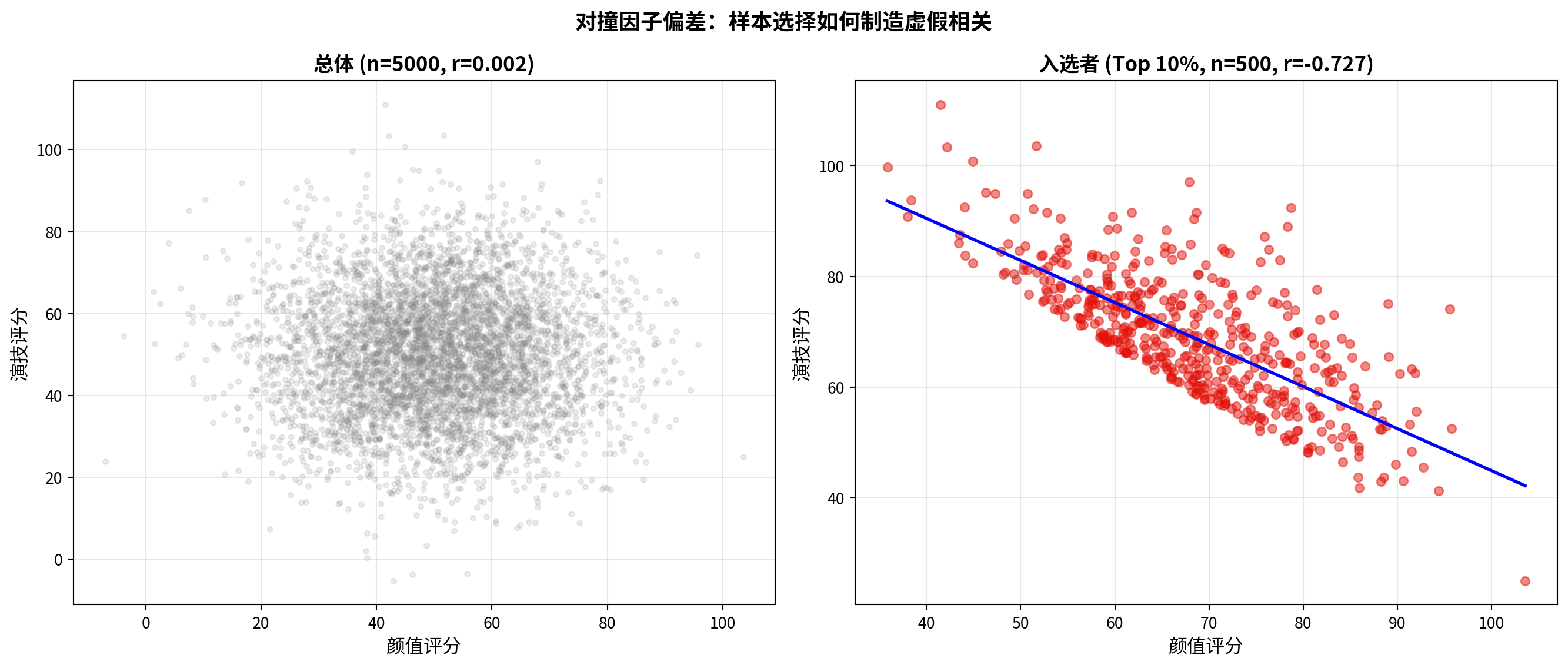
对撞因子对比图绘制完毕。下面输出数值证据与启示。
The collider bias comparison chart is complete. Below we output numerical evidence and insights.
# ========== 第6步:输出对撞因子偏差的数值证据与启示 ==========
# ========== Step 6: Output numerical evidence and insights on collider bias ==========
print(f'总体 (N={population_size}): r = {pop_r:.4f} (p = {pop_p:.4f})')  # 总体相关(≈0)
# Population correlation (≈ 0)
print(f'入选者 (Top 10%, n={is_selected.sum()}): r = {sel_r:.4f} (p = {sel_p:.4f})')  # 子样本相关(显著负)
# Subsample correlation (significantly negative)
print(f'\n启示:只分析"成功"样本(上市公司、学术明星等)')                 # 对撞因子的实际例子
# Practical examples of collider bias
print(f'可能观察到变量间的虚假相关——对撞因子偏差(Collider Bias)!')        # 核心警示
# Core warning: spurious correlations may arise — Collider Bias!
总体 (N=5000): r = 0.0021 (p = 0.8806)
入选者 (Top 10%, n=500): r = -0.7267 (p = 0.0000)
启示:只分析"成功"样本(上市公司、学术明星等)
可能观察到变量间的虚假相关——对撞因子偏差(Collider Bias)!运行结果和 图 8.6 生动地演示了对撞因子偏差的形成机制。在总体中(\(N = 5000\)),颜值与演技的相关系数 \(r = 0.0021\),\(p = 0.8806\),两个属性完全独立、无任何关联——这符合我们的预期。然而,一旦通过”综合得分前 10%“的选择机制对样本进行筛选(模拟”只有颜值或演技突出才能成为明星”),入选子样本(\(n = 500\))中两者的相关系数骤降至 \(r = -0.7267\),\(p \approx 0.0000\),呈现出极其显著的虚假负相关。其因果逻辑是:在入选者中,颜值特别高的人不需要很高的演技就能入选,而演技特别出色的人也不需要很高的颜值——这种选择造成了”此高彼低”的假象。在金融研究中,这一偏差同样常见:例如,只分析”上市公司”(存活偏差)、“成功的基金经理”或”论文被发表的研究”,都可能因对撞因子效应而导致变量间虚假相关的错误结论。
The results and 图 8.6 vividly demonstrate the mechanism behind collider bias. In the population (\(N = 5000\)), the correlation between attractiveness and acting skill is \(r = 0.0021\) with \(p = 0.8806\) — the two attributes are completely independent with no association, exactly as expected. However, once the sample is filtered through the selection mechanism of “top 10% by combined score” (simulating “only those with outstanding looks or acting talent can become celebrities”), the correlation in the selected subsample (\(n = 500\)) plummets to \(r = -0.7267\) with \(p \approx 0.0000\), exhibiting a highly significant spurious negative correlation. The causal logic is as follows: among those selected, individuals with exceptionally high attractiveness do not need very high acting skill to be selected, and those with exceptionally high acting skill do not need very high attractiveness — this selection process creates the illusion that “high on one means low on the other.” In financial research, this bias is equally prevalent: for example, analyzing only “listed companies” (survivorship bias), “successful fund managers,” or “published research studies” may all lead to erroneous conclusions of spurious correlations between variables due to the collider effect.