# ========== 导入所需库 ==========
# ========== Import required libraries ==========
import pandas as pd                # 数据分析核心库
                                   # Core library for data analysis
import numpy as np                 # 数值计算库
                                   # Library for numerical computation
from scipy import stats            # 统计检验函数库
                                   # Library for statistical testing functions
import matplotlib.pyplot as plt    # 数据可视化库
                                   # Library for data visualization
import platform                    # 操作系统平台检测
                                   # Library for OS platform detection

# ========== 第1步:设置中文字体 ==========
# ========== Step 1: Configure Chinese fonts ==========
if platform.system() == 'Linux':                                                        # 判断是否为Linux系统
                                                                                         # Check if running on Linux
    plt.rcParams['font.sans-serif'] = ['Source Han Serif SC', 'SimHei', 'DejaVu Sans']  # Linux字体列表
                                                                                         # Linux font list
else:                                                                                    # Windows系统
                                                                                         # Windows system
    plt.rcParams['font.sans-serif'] = ['SimHei', 'Microsoft YaHei']                     # Windows字体列表
                                                                                         # Windows font list
plt.rcParams['axes.unicode_minus'] = False                                               # 解决负号显示为方块的问题
                                                                                         # Fix minus sign display issue

# ========== 第2步:根据操作系统设置数据路径 ==========
# ========== Step 2: Set data path based on operating system ==========
if platform.system() == 'Linux':                                                # Linux平台
                                                                                 # Linux platform
    data_path = '/home/ubuntu/r2_data_mount/qiufei/data/stock'                  # Linux数据目录
                                                                                 # Linux data directory
else:                                                                            # Windows平台
                                                                                 # Windows platform
    data_path = 'C:/qiufei/data/stock'                                          # Windows数据目录
                                                                                 # Windows data directory

# ========== 第3步:读取本地财务数据和股票基本信息 ==========
# ========== Step 3: Read local financial data and stock basic information ==========
financial_statement_dataframe = pd.read_hdf(f'{data_path}/financial_statement.h5')  # 读取上市公司财务报表
                                                                                              # Read listed company financial statements
stock_basic_info_dataframe = pd.read_hdf(f'{data_path}/stock_basic_data.h5')        # 读取股票基本信息
                                                                                              # Read stock basic information

# ========== 第4步:筛选最近完整年度数据(2023年报) ==========
# ========== Step 4: Filter latest complete annual data (2023 annual report) ==========
latest_annual_report_dataframe = financial_statement_dataframe[  # 按条件筛选2023年年报数据
                                                                 # Filter 2023 annual report data by conditions
    (financial_statement_dataframe['quarter'].str.endswith('q4')) &       # 筛选第四季度(年报)
                                                                          # Filter Q4 (annual report)
    (financial_statement_dataframe['quarter'].str.startswith('2023'))     # 筛选2023年
                                                                          # Filter year 2023
].copy()                                                                  # 创建副本避免链式赋值警告
# Create copy to avoid chained assignment warning9 方差分析 (ANOVA)
方差分析(Analysis of Variance, ANOVA)是比较三个或更多组均值的统计方法。它由英国统计学家罗纳德·费希尔(Ronald Fisher)于20世纪初提出,是实验设计和统计推断的核心工具。ANOVA的核心思想是将数据的总变异分解为不同来源的变异,通过比较变异成分的相对大小来检验组间均值是否存在显著差异。
Analysis of Variance (ANOVA) is a statistical method for comparing the means of three or more groups. Developed by British statistician Ronald Fisher in the early 20th century, it is a core tool for experimental design and statistical inference. The central idea of ANOVA is to decompose the total variation in the data into variation from different sources, and to test whether the group means differ significantly by comparing the relative magnitudes of these variation components.
9.1 方差分析在行业研究与投资分析中的典型应用 (Typical Applications of ANOVA in Industry Research and Investment Analysis)
ANOVA的核心价值在于它能够同时比较多个组别的差异,而避免重复两两比较带来的第一类错误膨胀问题。以下展示其在中国金融研究中的核心应用。
The core value of ANOVA lies in its ability to compare differences across multiple groups simultaneously, while avoiding the Type I error inflation caused by repeated pairwise comparisons. The following demonstrates its key applications in Chinese financial research.
9.1.1 应用一:行业间盈利能力差异比较 (Application 1: Inter-Industry Profitability Comparison)
行业研究的基本问题是:不同行业的盈利能力是否存在显著差异?使用 financial_statement.h5 中的ROE数据,结合 stock_basic_data.h5 中的行业分类,对制造业、信息技术、金融、房地产、医药等多个行业的ROE进行单因素方差分析。如果F统计量显著,则说明行业归属对公司盈利能力有显著影响,进而使用事后多重比较(如Tukey HSD)识别具体哪些行业之间存在显著差异。
The fundamental question in industry research is: Do significant differences in profitability exist across industries? Using ROE data from financial_statement.h5 combined with industry classifications from stock_basic_data.h5, we perform one-way ANOVA on ROE across multiple industries such as manufacturing, information technology, finance, real estate, and pharmaceuticals. If the F-statistic is significant, it indicates that industry affiliation has a significant impact on firm profitability. Post-hoc multiple comparison tests (such as Tukey HSD) can then identify which specific pairs of industries differ significantly.
9.1.2 应用二:投资策略的多组别超额收益比较 (Application 2: Multi-Group Comparison of Strategy Excess Returns)
量化投资中,当需要同时比较多种策略(如价值策略、动量策略、质量策略、低波策略)的超额收益是否存在显著差异时,ANOVA是正确的工具。如果使用多次两两t检验,第一类错误率会急剧膨胀,导致错误地”发现”并不存在的策略差异——这是量化投资中”过拟合”(Overfitting)问题的统计学根源。
In quantitative investing, when one needs to simultaneously compare whether the excess returns of multiple strategies (e.g., value, momentum, quality, and low-volatility strategies) differ significantly, ANOVA is the appropriate tool. If multiple pairwise t-tests were used instead, the Type I error rate would inflate sharply, leading to the erroneous “discovery” of strategy differences that do not actually exist—this is the statistical root cause of the “overfitting” problem in quantitative investing.
9.1.3 应用三:地区经济发展差异分析 (Application 3: Regional Economic Development Disparity Analysis)
结合 stock_basic_data.h5 中的地区信息,将A股上市公司按省份分组(如上海、江苏、浙江、安徽、广东等),对其财务指标进行方差分析,可以实证检验不同地区的经济发展水平是否存在显著差异。这类分析对区域经济政策研究和投资区域配置策略具有重要参考价值。这一分析还可以结合 map 文件夹下的地理数据进行可视化展示。
By combining regional information from stock_basic_data.h5, A-share listed companies can be grouped by province (e.g., Shanghai, Jiangsu, Zhejiang, Anhui, Guangdong, etc.) and their financial indicators subjected to ANOVA, empirically testing whether significant differences in economic development levels exist across regions. This type of analysis is of great reference value for regional economic policy research and investment regional allocation strategies. The analysis can also be visualized using geographic data from the map folder.
9.1.4 为什么不能用多次t检验代替ANOVA? (Why Can’t Multiple t-Tests Replace ANOVA?)
当只有两个组时,我们可以使用独立样本t检验来比较均值。但当组数\(k \geq 3\)时,进行所有可能的两两t检验会带来严重问题:
When there are only two groups, we can use an independent samples t-test to compare means. However, when the number of groups \(k \geq 3\), performing all possible pairwise t-tests introduces serious problems:
检验次数过多: \(k\)个组需要进行\(\binom{k}{2} = \frac{k(k-1)}{2}\)次t检验
多重比较问题: 每次检验犯第一类错误的概率为\(\alpha\),多次检验后总体犯错概率急剧上升
Too many tests: \(k\) groups require \(\binom{k}{2} = \frac{k(k-1)}{2}\) t-tests
Multiple comparison problem: The probability of committing a Type I error is \(\alpha\) for each test, and after multiple tests, the overall probability of error increases dramatically
多重比较的第一类错误膨胀
Type I Error Inflation from Multiple Comparisons
假设每次检验的显著性水平为\(\alpha = 0.05\),进行\(m\)次独立检验时,至少犯一次第一类错误的概率如 式 9.1 所示:
Assuming a significance level of \(\alpha = 0.05\) for each test, when performing \(m\) independent tests, the probability of committing at least one Type I error is shown in 式 9.1:
\[ P(\text{至少一次错误}) = 1 - (1-\alpha)^m \tag{9.1}\]
对于\(k=4\)组的情况,需要进行\(\binom{4}{2}=6\)次两两比较:
For the case of \(k=4\) groups, \(\binom{4}{2}=6\) pairwise comparisons are needed:
\[ P = 1 - (1-0.05)^6 = 1 - 0.735 = 0.265 \]
这意味着即使所有组均值实际相等,我们也有26.5%的概率错误地认为至少有一对不相等!
This means that even if all group means are actually equal, there is a 26.5% probability that we would incorrectly conclude that at least one pair is unequal!
ANOVA通过一次综合检验巧妙地避免了这个问题,将总体第一类错误率控制在\(\alpha\)水平。
ANOVA cleverly avoids this problem through a single omnibus test, keeping the overall Type I error rate at the \(\alpha\) level.
9.2 从理论到实践:苦活累活 (The “Dirty Work”: From Theory to Practice)
ANOVA 最危险的地方在于它太容易”误用”了。
The most dangerous aspect of ANOVA is that it is all too easy to “misuse.”
9.2.1 事后诸葛亮 (Post-hoc Hacking)
如果你做了 ANOVA 发现显著,然后把所有组都两两比较一遍(Pairwise t-tests),直到找到那个 \(p < 0.05\) 的结果。
If you run ANOVA, find significance, and then perform all pairwise comparisons (Pairwise t-tests) until you find that \(p < 0.05\) result.
错误:你犯了”多重比较”错误。如果你做 20 次 t 检验,即使没有任何真实差异,你也有 \(64\%\) 的概率至少发现一个”显著”结果 (\(1 - 0.95^{20}\))。
对策:必须使用 Tukey HSD 或 Bonferroni 校正。不要裸奔!
Mistake: You have committed a “multiple comparisons” error. If you run 20 t-tests, even with no real differences, you have a \(64\%\) chance of finding at least one “significant” result (\(1 - 0.95^{20}\)).
Remedy: You must use Tukey HSD or Bonferroni correction. Don’t go unprotected!
9.2.2 假设的崩溃 (Assumption Breakdown)
正态性:ANOVA 对轻微的非正态性是稳健的(Robust),但对严重偏态(如对数正态分布)非常敏感。
方差齐性:这是 ANOVA 的死穴。如果一组方差大,一组方差小,F 检验会完全失效。
Normality: ANOVA is robust to mild non-normality, but is very sensitive to severe skewness (e.g., log-normal distributions).
Homogeneity of Variances: This is ANOVA’s Achilles’ heel. If one group has a large variance and another has a small variance, the F-test will completely break down.
建议:在 Python 中,Default to Welch’s ANOVA (
pingouin.welch_anova)。它不需要方差齐性假设,且在方差齐性时依然高效。
Recommendation: In Python, default to Welch’s ANOVA (
pingouin.welch_anova). It does not require the homogeneity of variances assumption, and remains efficient even when variances are equal.
9.3 单因素方差分析 (One-Way ANOVA)
9.3.1 模型设定 (Model Specification)
单因素方差分析的统计模型如 式 9.2 所示:
The statistical model for one-way ANOVA is shown in 式 9.2:
\[ Y_{ij} = \mu + \tau_i + \varepsilon_{ij}, \quad i=1,2,...,k; \quad j=1,2,...,n_i \tag{9.2}\]
其中:
Where:
\(Y_{ij}\): 第\(i\)组第\(j\)个观测值
\(\mu\): 总体均值(grand mean)
\(\tau_i\): 第\(i\)组的处理效应(treatment effect),满足\(\sum_{i=1}^k n_i \tau_i = 0\)
\(\varepsilon_{ij} \sim N(0, \sigma^2)\): 随机误差项,假设独立同分布
\(k\): 组数
\(n_i\): 第\(i\)组的样本量
\(N = \sum_{i=1}^k n_i\): 总样本量
\(Y_{ij}\): The \(j\)-th observation in the \(i\)-th group
\(\mu\): The grand mean
\(\tau_i\): The treatment effect of the \(i\)-th group, satisfying \(\sum_{i=1}^k n_i \tau_i = 0\)
\(\varepsilon_{ij} \sim N(0, \sigma^2)\): Random error term, assumed to be independently and identically distributed
\(k\): Number of groups
\(n_i\): Sample size of the \(i\)-th group
\(N = \sum_{i=1}^k n_i\): Total sample size
9.3.2 假设检验 (Hypothesis Testing)
原假设 \(H_0\): \(\tau_1 = \tau_2 = ... = \tau_k = 0\)
Null Hypothesis \(H_0\): \(\tau_1 = \tau_2 = ... = \tau_k = 0\)
等价于: \(\mu_1 = \mu_2 = ... = \mu_k\) (所有组均值相等)
Equivalently: \(\mu_1 = \mu_2 = ... = \mu_k\) (all group means are equal)
备择假设 \(H_1\): 至少有一个\(\tau_i \neq 0\)
Alternative Hypothesis \(H_1\): At least one \(\tau_i \neq 0\)
等价于: 至少有一对组均值不相等
Equivalently: At least one pair of group means are unequal
9.3.3 变异分解的数学推导 (Mathematical Derivation of Variation Decomposition)
ANOVA的核心是将总变异分解为组间变异和组内变异。令:
The core of ANOVA is decomposing total variation into between-group variation and within-group variation. Let:
\(\bar{Y}_{i.} = \frac{1}{n_i}\sum_{j=1}^{n_i} Y_{ij}\): 第\(i\)组的样本均值
\(\bar{Y}_{..} = \frac{1}{N}\sum_{i=1}^k \sum_{j=1}^{n_i} Y_{ij}\): 总样本均值
\(\bar{Y}_{i.} = \frac{1}{n_i}\sum_{j=1}^{n_i} Y_{ij}\): The sample mean of the \(i\)-th group
\(\bar{Y}_{..} = \frac{1}{N}\sum_{i=1}^k \sum_{j=1}^{n_i} Y_{ij}\): The overall sample mean
平方和分解的代数证明
Algebraic Proof of the Sum of Squares Decomposition
这是一个优美的恒等式,依赖于交叉项的消失。
This is an elegant identity that relies on the vanishing of the cross term.
\[ Y_{ij} - \bar{Y}_{..} = (\bar{Y}_{i.} - \bar{Y}_{..}) + (Y_{ij} - \bar{Y}_{i.}) \]
两边平方并求和:
Squaring both sides and summing:
\[ \sum_{i,j}(Y_{ij} - \bar{Y}_{..})^2 = \sum_{i,j}(\bar{Y}_{i.} - \bar{Y}_{..})^2 + \sum_{i,j}(Y_{ij} - \bar{Y}_{i.})^2 + 2\sum_{i=1}^k \sum_{j=1}^{n_i}(\bar{Y}_{i.} - \bar{Y}_{..})(Y_{ij} - \bar{Y}_{i.}) \]
看交叉项:
Examining the cross term:
\[ 2\sum_{i=1}^k (\bar{Y}_{i.} - \bar{Y}_{..}) \underbrace{\sum_{j=1}^{n_i}(Y_{ij} - \bar{Y}_{i.})}_{0} = 0 \]
因为 \(\sum_{j=1}^{n_i}(Y_{ij} - \bar{Y}_{i.}) = \sum Y_{ij} - n_i \bar{Y}_{i.} = n_i \bar{Y}_{i.} - n_i \bar{Y}_{i.} = 0\)。即组内偏差之和必为零。
Because \(\sum_{j=1}^{n_i}(Y_{ij} - \bar{Y}_{i.}) = \sum Y_{ij} - n_i \bar{Y}_{i.} = n_i \bar{Y}_{i.} - n_i \bar{Y}_{i.} = 0\). That is, the sum of within-group deviations is always zero.
几何解释(毕达哥拉斯定理):
Geometric Interpretation (Pythagorean Theorem):
我们将所有观测值看作一个 \(N\) 维向量 \(\mathbf{y}\)。
We view all observations as an \(N\)-dimensional vector \(\mathbf{y}\).
总变异向量 \(\mathbf{y} - \bar{y}\mathbf{1}\)
组间变异向量(投影到组均值空间)
组内变异向量(残差空间)
Total variation vector \(\mathbf{y} - \bar{y}\mathbf{1}\)
Between-group variation vector (projection onto the group mean space)
Within-group variation vector (residual space)
这两个子空间是正交的,因此平方和满足勾股定理:
These two subspaces are orthogonal, so the sums of squares satisfy the Pythagorean theorem:
\[ \|\text{Total}\|^2 = \|\text{Between}\|^2 + \|\text{Within}\|^2 \]
即 \(SST = SSB + SSW\)。
That is, \(SST = SSB + SSW\).
三个平方和的含义如 表 9.1 所示:
The meanings of the three sums of squares are shown in 表 9.1:
| 平方和 | 名称 | 自由度 | 度量内容 |
|---|---|---|---|
| \(SST\) | 总平方和 (Total) | \(N-1\) | 数据的总变异 |
| \(SSB\) | 组间平方和 (Between) | \(k-1\) | 组均值之间的变异 |
| \(SSW\) | 组内平方和 (Within) | \(N-k\) | 组内个体间的变异 |
9.3.4 均方与F统计量 (Mean Squares and the F-Statistic)
均方(Mean Square)是平方和除以相应的自由度,如 式 9.3 所示:
The Mean Square (MS) is the sum of squares divided by the corresponding degrees of freedom, as shown in 式 9.3:
\[ MSB = \frac{SSB}{k-1}, \quad MSW = \frac{SSW}{N-k} \tag{9.3}\]
F统计量是组间均方与组内均方的比值,如 式 9.4 所示:
The F-statistic is the ratio of the between-group mean square to the within-group mean square, as shown in 式 9.4:
\[ F = \frac{MSB}{MSW} \tag{9.4}\]
F统计量抽样分布的推导
Derivation of the Sampling Distribution of the F-Statistic
在\(H_0\)成立(所有组均值相等)的条件下,可以证明:
Under \(H_0\) (all group means are equal), it can be shown that:
\(\frac{SSW}{\sigma^2} \sim \chi^2(N-k)\)
\(\frac{SSB}{\sigma^2} \sim \chi^2(k-1)\)
\(SSB\)与\(SSW\)相互独立
\(\frac{SSW}{\sigma^2} \sim \chi^2(N-k)\)
\(\frac{SSB}{\sigma^2} \sim \chi^2(k-1)\)
\(SSB\) and \(SSW\) are mutually independent
根据F分布的定义(两个独立卡方变量除以各自自由度的比值),可得 式 9.5:
By the definition of the F-distribution (the ratio of two independent chi-squared variables each divided by their respective degrees of freedom), we obtain 式 9.5:
\[ F = \frac{SSB/(k-1)}{SSW/(N-k)} = \frac{MSB}{MSW} \sim F(k-1, N-k) \tag{9.5}\]
直观理解:
Intuitive Understanding:
当\(H_0\)成立时,\(MSB\)和\(MSW\)都是\(\sigma^2\)的无偏估计,所以\(F \approx 1\)
当\(H_1\)成立时,组间存在真实差异,\(MSB\)会系统性地大于\(MSW\),导致\(F > 1\)
\(F\)值越大,拒绝\(H_0\)的证据越强
When \(H_0\) holds, both \(MSB\) and \(MSW\) are unbiased estimates of \(\sigma^2\), so \(F \approx 1\)
When \(H_1\) holds, real differences exist between groups, and \(MSB\) will be systematically larger than \(MSW\), leading to \(F > 1\)
The larger the \(F\) value, the stronger the evidence against \(H_0\)
9.3.5 期望均方 (Expected Mean Squares)
理解为什么F统计量有效的关键是计算期望均方(式 9.6 和 式 9.7):
The key to understanding why the F-statistic works is to compute the expected mean squares (式 9.6 and 式 9.7):
\[ E(MSW) = \sigma^2 \tag{9.6}\]
\[ E(MSB) = \sigma^2 + \frac{\sum_{i=1}^k n_i \tau_i^2}{k-1} \tag{9.7}\]
期望均方的含义
Interpretation of the Expected Mean Squares
\(MSW\)总是\(\sigma^2\)的无偏估计,无论\(H_0\)是否成立
只有当\(H_0\)成立(即所有\(\tau_i = 0\))时,\(MSB\)才是\(\sigma^2\)的无偏估计
当存在处理效应时,\(E(MSB) > \sigma^2\),导致\(F\)值增大
\(MSW\) is always an unbiased estimate of \(\sigma^2\), regardless of whether \(H_0\) holds
Only when \(H_0\) holds (i.e., all \(\tau_i = 0\)) is \(MSB\) an unbiased estimate of \(\sigma^2\)
When treatment effects exist, \(E(MSB) > \sigma^2\), causing the \(F\) value to increase
这就是为什么我们使用\(F = MSB/MSW\)作为检验统计量:在\(H_0\)下\(E(F) \approx 1\),在\(H_1\)下\(E(F) > 1\)。
This is why we use \(F = MSB/MSW\) as the test statistic: under \(H_0\), \(E(F) \approx 1\); under \(H_1\), \(E(F) > 1\).
9.4 案例:不同行业上市公司盈利能力比较 (Case Study: Profitability Comparison Across Industries for Listed Companies)
什么是行业间盈利能力的差异比较?
What Is an Inter-Industry Profitability Comparison?
在行业研究和投资组合管理中,一个基本问题是:不同行业的企业盈利能力是否存在显著差异?例如,金融业的ROE是否显著高于制造业?这种跨行业比较对于行业配置策略、产业政策制定和企业竞争力分析都具有重要的指导价值。
In industry research and portfolio management, a fundamental question is: Do significant differences in profitability exist across industries? For example, is the banking sector’s ROE significantly higher than that of manufacturing? Such cross-industry comparisons are of great guiding value for sector allocation strategies, industrial policy formulation, and corporate competitiveness analysis.
当我们需要同时比较三个及以上组别的均值差异时,方差分析(ANOVA)是比多次两两t检验更为科学的方法:它通过将总变异分解为组间变异和组内变异,用一个F检验就能判断各组均值是否全部相等。下面使用本地中国A股上市公司财务数据,比较不同行业的净资产收益率(ROE)是否存在显著差异,结果如 表 9.2 所示。
When we need to compare the mean differences of three or more groups simultaneously, ANOVA is a more scientifically sound method than multiple pairwise t-tests: by decomposing total variation into between-group and within-group variation, a single F-test determines whether all group means are equal. Below we use local Chinese A-share listed company financial data to compare whether significant differences in Return on Equity (ROE) exist across industries, with results shown in 表 9.2.
年报数据筛选完成。下面合并行业信息,计算ROE,并筛选长三角地区代表性行业数据。
Annual report data filtering is complete. Next we merge industry information, calculate ROE, and filter representative industry data for the Yangtze River Delta region.
# ========== 第5步:合并行业和省份信息 ==========
# ========== Step 5: Merge industry and province information ==========
latest_annual_report_dataframe = latest_annual_report_dataframe.merge(  # 合并行业与省份基本信息
                                                                        # Merge industry and province basic information
    stock_basic_info_dataframe[['order_book_id', 'industry_name', 'province']],  # 选取行业名称和省份
                                                                                  # Select industry name and province
    on='order_book_id',                                                           # 按股票代码匹配
                                                                                  # Match by stock code
    how='left'                                                                    # 左连接保留所有财务数据
                                                                                  # Left join to retain all financial data
)

# ========== 第6步:计算净资产收益率(ROE) ==========
# ========== Step 6: Calculate Return on Equity (ROE) ==========
latest_annual_report_dataframe['roe'] = latest_annual_report_dataframe['net_profit'] / latest_annual_report_dataframe['total_equity'] * 100  # ROE = 净利润/净资产 × 100%
                                                                                                                                              # ROE = Net Profit / Total Equity × 100%

# ========== 第7步:聚焦长三角地区企业 ==========
# ========== Step 7: Focus on Yangtze River Delta enterprises ==========
yangtze_river_delta_areas_list = ['上海市', '江苏省', '浙江省', '安徽省']          # 定义长三角四省市
                                                                                   # Define the four YRD provinces/municipalities
yangtze_river_delta_dataframe = latest_annual_report_dataframe[latest_annual_report_dataframe['province'].isin(yangtze_river_delta_areas_list)].copy()  # 筛选长三角地区
                                                                                                                                                         # Filter YRD region
长三角地区企业数据筛选完毕。下面定义代表性行业映射并进行最终数据清洗。
Yangtze River Delta enterprise data filtering is complete. Next we define the representative industry mapping and perform final data cleaning.
# ========== 第8步:定义代表性行业及显示名称映射 ==========
# ========== Step 8: Define representative industries and display name mapping ==========
industry_display_mapping = {                                           # 国统局行业分类名 → 简称
                                                                       # NBS industry classification name → abbreviation
    '货币金融服务': '银行',                                             # 银行业
                                                                       # Banking sector
    '医药制造业': '医药生物',                                           # 医药行业
                                                                       # Pharmaceutical sector
    '计算机、通信和其他电子设备制造业': '电子',                          # 电子行业
                                                                       # Electronics sector
    '专用设备制造业': '机械设备',                                       # 机械设备行业
                                                                       # Machinery and equipment sector
    '软件和信息技术服务业': '计算机',                                   # 计算机行业
                                                                       # Computer/IT sector
}
representative_industries_list = list(industry_display_mapping.keys())  # 提取国统局原始行业名称列表
                                                                        # Extract list of NBS original industry names

# ========== 第9步:筛选数据并去除异常值 ==========
# ========== Step 9: Filter data and remove outliers ==========
selected_industry_data_dataframe = yangtze_river_delta_dataframe[  # 多条件筛选目标行业有效数据
                                                                    # Multi-condition filter for valid target industry data
    (yangtze_river_delta_dataframe['industry_name'].isin(representative_industries_list)) &  # 筛选目标行业
                                                                                              # Filter target industries
    (yangtze_river_delta_dataframe['roe'].notna()) &                                         # 排除ROE缺失值
                                                                                              # Exclude missing ROE values
    (yangtze_river_delta_dataframe['roe'] > -50) &  # 去除极端亏损(ROE低于-50%)
                                                     # Remove extreme losses (ROE below -50%)
    (yangtze_river_delta_dataframe['roe'] < 50)     # 去除极端盈利(ROE高于50%)
                                                     # Remove extreme profits (ROE above 50%)
].copy()                                             # 创建副本
                                                     # Create a copy
完成数据准备后,我们对各行业的ROE进行描述性统计分析,并执行单因素方差分析(ANOVA)来检验行业间ROE的差异是否显著:
After completing data preparation, we perform descriptive statistical analysis of ROE for each industry and execute a one-way ANOVA to test whether the differences in ROE across industries are significant:
print('=== 长三角地区不同行业上市公司ROE分析 ===\n')  # 输出分析标题
                                                        # Print analysis title

# ========== 第10步:各行业ROE描述性统计 ==========
# ========== Step 10: Descriptive statistics of ROE by industry ==========
print('各行业ROE描述性统计:')                         # 提示输出内容
                                                       # Prompt output content
industry_descriptive_statistics = selected_industry_data_dataframe.groupby('industry_name')['roe'].agg(['count', 'mean', 'std', 'min', 'max'])  # 按行业分组计算统计指标
                                                                                                                                                  # Compute statistics grouped by industry
industry_descriptive_statistics.columns = ['样本量', '均值(%)', '标准差', '最小值', '最大值']  # 重命名列为中文
                                                                                                # Rename columns to Chinese
print(industry_descriptive_statistics.round(2))       # 输出保留两位小数的描述统计表
                                                       # Print descriptive statistics rounded to 2 decimals
=== 长三角地区不同行业上市公司ROE分析 ===
各行业ROE描述性统计:
样本量 均值(%) 标准差 最小值 最大值
industry_name
专用设备制造业 156 6.38 9.90 -49.94 33.51
医药制造业 96 3.07 11.18 -41.15 35.11
计算机、通信和其他电子设备制造业 195 2.35 11.13 -46.48 33.88
货币金融服务 18 10.63 2.23 5.11 14.90
软件和信息技术服务业 105 0.82 12.01 -43.92 32.37描述统计结果显示五个行业的ROE存在明显分化。银行业(货币金融服务)样本量最小(n=18)但ROE均值最高(10.63%),标准差仅2.23%,说明银行业盈利稳定且水平较高。机械设备(专用设备制造业)n=156,均值6.38%,标准差9.90%。医药(医药制造业)n=96,均值3.07%,标准差11.18%。电子(计算机、通信和其他电子设备制造业)n=195,均值2.35%,标准差11.13%。计算机(软件和信息技术服务业)n=105,均值仅0.82%,标准差12.01%,离散程度最大。总体来看,银行业ROE明显高于其他行业,而计算机行业ROE最低且波动最大。下面准备分组数据并执行单因素方差分析。
The descriptive statistics reveal a clear differentiation in ROE across the five industries. Banking (Monetary and Financial Services) has the smallest sample size (n=18) but the highest mean ROE (10.63%), with a standard deviation of only 2.23%, indicating stable and high profitability. Machinery and Equipment (Special-Purpose Equipment Manufacturing) has n=156, a mean of 6.38%, and a standard deviation of 9.90%. Pharmaceuticals (Pharmaceutical Manufacturing) has n=96, a mean of 3.07%, and a standard deviation of 11.18%. Electronics (Computer, Communications, and Other Electronic Equipment Manufacturing) has n=195, a mean of 2.35%, and a standard deviation of 11.13%. Computer/IT (Software and Information Technology Services) has n=105, a mean of only 0.82%, and the largest standard deviation of 12.01%. Overall, banking ROE is significantly higher than other industries, while the computer/IT sector has the lowest ROE with the greatest volatility. Next we prepare grouped data and execute a one-way ANOVA.
# ========== 第11步:准备ANOVA分组数据 ==========
# ========== Step 11: Prepare ANOVA grouped data ==========
industry_roe_data_groups = []                          # 初始化存储各行业ROE数组的列表
                                                       # Initialize list to store ROE arrays by industry
industry_names_list = []                               # 初始化存储行业简称的列表
                                                       # Initialize list to store industry abbreviations
for nbs_industry_name in representative_industries_list:  # 遍历各代表性行业
                                                           # Iterate over each representative industry
    single_industry_roe_array = selected_industry_data_dataframe[selected_industry_data_dataframe['industry_name'] == nbs_industry_name]['roe'].values  # 提取该行业ROE数组
                                                                                                                                                         # Extract ROE array for this industry
    if len(single_industry_roe_array) >= 5:  # 确保每组样本量≥5
                                              # Ensure each group has sample size >= 5
        industry_roe_data_groups.append(single_industry_roe_array)      # 添加ROE数组到分组列表
                                                                         # Append ROE array to grouped list
        industry_names_list.append(industry_display_mapping.get(nbs_industry_name, nbs_industry_name))  # 添加行业简称
                                                                                                         # Append industry abbreviation

# ========== 第12步:执行单因素方差分析并输出结论 ==========
# ========== Step 12: Execute one-way ANOVA and output conclusions ==========
anova_f_statistic, anova_p_value = stats.f_oneway(*industry_roe_data_groups)  # 调用scipy进行单因素ANOVA
                                                                                # Call scipy to perform one-way ANOVA

print(f'\n=== 单因素方差分析结果 ===')                 # 输出结果标题
                                                        # Print result title
print(f'F统计量: {anova_f_statistic:.4f}')             # 输出F统计量
                                                        # Print F-statistic
print(f'p值: {anova_p_value:.6f}')                     # 输出p值
                                                        # Print p-value
print(f'显著性水平: α = 0.05')                         # 输出显著性水平
                                                        # Print significance level

if anova_p_value < 0.05:                                # 判断是否拒绝原假设
                                                         # Determine whether to reject the null hypothesis
    print(f'\n结论: 拒绝原假设 (p = {anova_p_value:.4f} < 0.05)')      # p值小于0.05的结论
                                                                         # Conclusion when p-value < 0.05
    print('不同行业的ROE存在显著差异')                  # 行业间ROE显著不同
                                                         # ROE differs significantly across industries
else:                                                    # 不拒绝原假设
                                                         # Do not reject the null hypothesis
    print(f'\n结论: 不能拒绝原假设 (p = {anova_p_value:.4f} >= 0.05)')  # p值大于等于0.05的结论
                                                                          # Conclusion when p-value >= 0.05
    print('不同行业的ROE差异不显著')                    # 行业间ROE差异不显著
                                                         # ROE does not differ significantly across industries
=== 单因素方差分析结果 ===
F统计量: 6.9040
p值: 0.000020
显著性水平: α = 0.05

结论: 拒绝原假设 (p = 0.0000 < 0.05)
不同行业的ROE存在显著差异
单因素方差分析结果显示,F统计量=6.9040,p值=0.000020,远小于0.05的显著性水平。因此拒绝原假设,结论是不同行业的ROE存在显著差异。这一结果与描述统计中观察到的行业间ROE分化是一致的。
The one-way ANOVA results show that the F-statistic = 6.9040 and p-value = 0.000020, far below the 0.05 significance level. We therefore reject the null hypothesis, concluding that ROE differs significantly across industries. This result is consistent with the inter-industry ROE differentiation observed in the descriptive statistics.
图 9.1 直观展示了各行业ROE的分布差异,箱线图中可以清楚看到不同行业间的中位数和离散程度差异。
图 9.1 visually displays the distributional differences in ROE across industries; the box plots clearly show the differences in medians and dispersion among different industries.
# ========== 第1步:创建1×2子图画布 ==========
# ========== Step 1: Create a 1×2 subplot canvas ==========
matplot_figure, matplot_axes_array = plt.subplots(1, 2, figsize=(14, 6))  # 创建1行2列子图
                                                                           # Create 1-row, 2-column subplots

# ========== 第2步:绘制各行业ROE箱线图(左图) ==========
# ========== Step 2: Draw ROE box plots by industry (left panel) ==========
boxplot_axes = matplot_axes_array[0]                                      # 获取左侧子图轴
                                                                           # Get the left subplot axes
boxplot_object = boxplot_axes.boxplot(industry_roe_data_groups, labels=industry_names_list, patch_artist=True, showmeans=True)  # 绘制箱线图,填充颜色并显示均值
                                                                                                                                 # Draw box plot with filled colors and mean markers

box_fill_colors_list = ['#E3120B', '#2C3E50', '#008080', '#F0A700', '#8E9EAA']  # 定义5种行业配色
                                                                                  # Define 5 industry colors
for box_patch_item, single_color_code in zip(boxplot_object['boxes'], box_fill_colors_list):  # 逐箱体上色
                                                                                                # Color each box
    box_patch_item.set_facecolor(single_color_code)                        # 设置填充颜色
                                                                            # Set fill color
    box_patch_item.set_alpha(0.7)                                          # 设置透明度
                                                                            # Set transparency

boxplot_axes.axhline(y=0, color='gray', linestyle='--', alpha=0.5)        # 添加ROE=0的参考线
                                                                           # Add ROE=0 reference line
boxplot_axes.set_ylabel('ROE (%)', fontsize=12)                            # 设置Y轴标签
                                                                           # Set Y-axis label
boxplot_axes.set_xlabel('行业', fontsize=12)                               # 设置X轴标签
                                                                           # Set X-axis label
boxplot_axes.set_title('各行业ROE箱线图', fontsize=14)                     # 设置子图标题
                                                                           # Set subplot title
boxplot_axes.grid(True, axis='y', alpha=0.3)                               # 添加Y轴网格线
                                                                           # Add Y-axis grid lines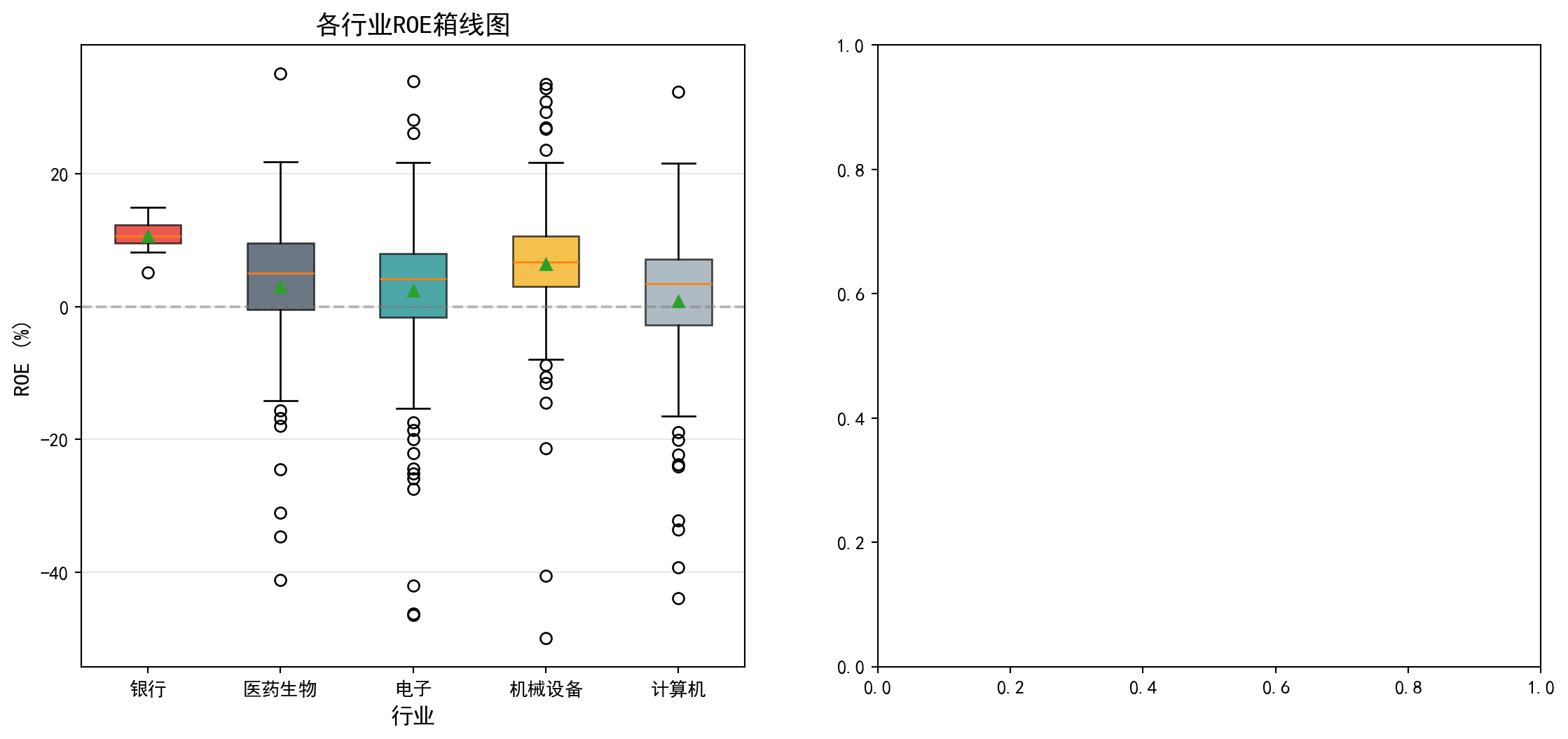
左侧箱线图已绘制完成,可以直观地看到各行业ROE的中位数、四分位距和异常值。从图中可以看出,银行业的箱体位置明显高于其他行业且非常紧凑,反映出银行业ROE集中在较高水平;计算机行业箱体位置最低且分布范围最广;各行业均存在一些异常值(离群点),表明个别公司ROE偏离行业整体水平较大。接下来,我们在右侧子图中绘制各行业ROE均值及其95%置信区间的误差棒图,以更精确地比较各组均值的差异及其统计不确定性。
The left box plot is now complete, intuitively showing the median, interquartile range, and outliers for each industry’s ROE. The chart reveals that the banking sector’s box is positioned significantly higher than other industries and is very compact, reflecting that banking ROE is concentrated at a higher level; the computer/IT sector’s box is positioned lowest with the widest spread; all industries have some outliers, indicating that individual company ROE deviates substantially from their industry’s overall level. Next, we draw an error bar plot of each industry’s mean ROE with 95% confidence intervals in the right subplot, to more precisely compare the differences in group means and their statistical uncertainty.
# ========== 第3步:绘制均值及95%置信区间图(右图) ==========
# ========== Step 3: Draw mean and 95% confidence interval plot (right panel) ==========
errorbar_axes = matplot_axes_array[1]                                      # 获取右侧子图轴
                                                                           # Get the right subplot axes
group_means_list = [np.mean(g) for g in industry_roe_data_groups]          # 计算各组均值
                                                                           # Calculate group means
group_std_devs_list = [np.std(g) for g in industry_roe_data_groups]        # 计算各组标准差
                                                                           # Calculate group standard deviations
group_sample_sizes_list = [len(g) for g in industry_roe_data_groups]       # 计算各组样本量
                                                                           # Calculate group sample sizes
group_confidence_intervals_list = [1.96 * s / np.sqrt(n) for s, n in zip(group_std_devs_list, group_sample_sizes_list)]  # 计算95%置信区间半宽
                                                                                                                           # Calculate 95% CI half-width

x_axis_positions = range(len(industry_names_list))                         # 生成X轴位置序列
                                                                           # Generate X-axis position sequence
errorbar_axes.errorbar(x_axis_positions, group_means_list, yerr=group_confidence_intervals_list, fmt='o', capsize=5, capthick=2,  # 配置误差棒图的样式参数
                                                                                                                                    # Configure error bar style parameters
             markersize=10, color='#E3120B', ecolor='#2C3E50')            # 绘制带误差棒的均值点
                                                                           # Draw mean points with error bars
errorbar_axes.axhline(y=np.mean([np.mean(g) for g in industry_roe_data_groups]), color='gray',  # 绘制总体均值水平参考线
                                                                                                  # Draw overall mean reference line
            linestyle='--', alpha=0.5, label='总体均值')                   # 添加总体均值参考线
                                                                           # Add overall mean reference line
errorbar_axes.set_xticks(x_axis_positions)                                 # 设置X轴刻度位置
                                                                           # Set X-axis tick positions
errorbar_axes.set_xticklabels(industry_names_list)                         # 设置X轴刻度标签
                                                                           # Set X-axis tick labels
errorbar_axes.set_ylabel('ROE均值 (%)', fontsize=12)                       # 设置Y轴标签
                                                                           # Set Y-axis label
errorbar_axes.set_xlabel('行业', fontsize=12)                              # 设置X轴标签
                                                                           # Set X-axis label
errorbar_axes.set_title('各行业ROE均值及95%置信区间', fontsize=14)          # 设置子图标题
                                                                           # Set subplot title
errorbar_axes.grid(True, axis='y', alpha=0.3)                              # 添加Y轴网格线
                                                                           # Add Y-axis grid lines
errorbar_axes.legend()                                                     # 显示图例
                                                                           # Show legend

# ========== 第4步:调整布局并显示图形 ==========
# ========== Step 4: Adjust layout and display figure ==========
plt.tight_layout()                                                         # 自动调整子图间距
                                                                           # Automatically adjust subplot spacing
plt.show()                                                                 # 显示图形
                                                                           # Display figure
<Figure size 672x480 with 0 Axes>9.4.1 手工计算ANOVA表 (Manually Computing the ANOVA Table)
为了深入理解ANOVA的计算过程,我们手工构建ANOVA表(表 9.3):
To deeply understand the ANOVA computation process, we manually construct the ANOVA table (表 9.3):
# ========== 第1步:合并所有组数据并计算总体均值 ==========
# ========== Step 1: Concatenate all group data and compute the grand mean ==========
concatenated_roe_array = np.concatenate(industry_roe_data_groups)   # 将各行业ROE数组合并为一个总数组
                                                                     # Concatenate ROE arrays from all industries into one
overall_grand_mean = np.mean(concatenated_roe_array)                # 计算所有样本的总体均值(Grand Mean)
                                                                     # Compute the grand mean of all samples
total_sample_size = len(concatenated_roe_array)                     # 计算总样本量N
                                                                     # Compute total sample size N
total_group_count = len(industry_roe_data_groups)                   # 计算组数k
                                                                     # Compute number of groups k

# ========== 第2步:计算三个平方和(SST/SSB/SSW) ==========
# ========== Step 2: Compute the three sums of squares (SST/SSB/SSW) ==========
total_sum_of_squares = np.sum((concatenated_roe_array - overall_grand_mean)**2)                              # SST: 总平方和 = Σ(Yij - Ȳ..)²
                                                                                                              # SST: Total Sum of Squares = Σ(Yij - Ȳ..)²
between_group_sum_of_squares = sum(len(g) * (np.mean(g) - overall_grand_mean)**2 for g in industry_roe_data_groups)  # SSB: 组间平方和 = Σni(Ȳi. - Ȳ..)²
                                                                                                                       # SSB: Between-Group Sum of Squares = Σni(Ȳi. - Ȳ..)²
within_group_sum_of_squares = sum(np.sum((g - np.mean(g))**2) for g in industry_roe_data_groups)             # SSW: 组内平方和 = ΣΣ(Yij - Ȳi.)²
                                                                                                              # SSW: Within-Group Sum of Squares = ΣΣ(Yij - Ȳi.)²

# ========== 第3步:计算自由度 ==========
# ========== Step 3: Compute degrees of freedom ==========
degrees_of_freedom_between = total_group_count - 1                  # 组间自由度 = k - 1
                                                                     # Between-group df = k - 1
degrees_of_freedom_within = total_sample_size - total_group_count   # 组内自由度 = N - k
                                                                     # Within-group df = N - k
degrees_of_freedom_total = total_sample_size - 1                    # 总自由度 = N - 1
                                                                     # Total df = N - 1

# ========== 第4步:计算均方(MS) ==========
# ========== Step 4: Compute Mean Squares (MS) ==========
mean_square_between = between_group_sum_of_squares / degrees_of_freedom_between  # MSB = SSB / (k-1)
                                                                                   # MSB = SSB / (k-1)
mean_square_within = within_group_sum_of_squares / degrees_of_freedom_within     # MSW = SSW / (N-k)
                                                                                   # MSW = SSW / (N-k)
平方和与均方的计算已完成。组间平方和(SSB)、组内平方和(SSW)和总平方和(SST)构成了ANOVA分解的基础。接下来将利用这些中间结果计算F统计量和p值,并构建完整的ANOVA汇总表。
The computation of sums of squares and mean squares is complete. The Between-Group Sum of Squares (SSB), Within-Group Sum of Squares (SSW), and Total Sum of Squares (SST) form the foundation of the ANOVA decomposition. Next, we use these intermediate results to compute the F-statistic and p-value, and construct the complete ANOVA summary table.
# ========== 第5步:计算F统计量和p值 ==========
# ========== Step 5: Compute F-statistic and p-value ==========
calculated_f_ratio = mean_square_between / mean_square_within                    # F = MSB / MSW
                                                                                  # F = MSB / MSW
manual_calculated_p_value = 1 - stats.f.cdf(calculated_f_ratio, degrees_of_freedom_between, degrees_of_freedom_within)  # 从F分布累积函数计算p值
                                                                                                                          # Compute p-value from the F-distribution CDF

# ========== 第6步:构建ANOVA表并输出 ==========
# ========== Step 6: Construct ANOVA table and output ==========
anova_results_dataframe = pd.DataFrame({                            # 创建ANOVA汇总表
                                                                     # Create ANOVA summary table
    '来源': ['组间 (Between)', '组内 (Within)', '总计 (Total)'],    # 变异来源
                                                                     # Sources of variation
    '平方和 (SS)': [between_group_sum_of_squares, within_group_sum_of_squares, total_sum_of_squares],  # 三个平方和
                                                                                                         # Three sums of squares
    '自由度 (df)': [degrees_of_freedom_between, degrees_of_freedom_within, degrees_of_freedom_total],  # 三个自由度
                                                                                                         # Three degrees of freedom
    '均方 (MS)': [mean_square_between, mean_square_within, np.nan],  # 均方(总计行无均方)
                                                                      # Mean squares (no MS for total row)
    'F值': [calculated_f_ratio, np.nan, np.nan],                     # F统计量(仅组间行)
                                                                      # F-statistic (between row only)
    'p值': [manual_calculated_p_value, np.nan, np.nan]               # p值(仅组间行)
                                                                      # p-value (between row only)
})

print('=== ANOVA表 ===')                                            # 输出表标题
                                                                     # Print table title
print(anova_results_dataframe.to_string(index=False))               # 以无索引格式输出ANOVA表
                                                                     # Print ANOVA table without index

# ========== 第7步:验证平方和分解 SST = SSB + SSW ==========
# ========== Step 7: Verify sum of squares decomposition SST = SSB + SSW ==========
print(f'\n验证平方和分解: SST = {total_sum_of_squares:.2f}, SSB + SSW = {between_group_sum_of_squares + within_group_sum_of_squares:.2f}')  # 验证等式
                                                                                                                                                # Verify the identity
print(f'差异: {abs(total_sum_of_squares - between_group_sum_of_squares - within_group_sum_of_squares):.10f} (浮点误差)')  # 输出浮点误差
                                                                                                                            # Print floating-point error
=== ANOVA表 ===
来源 平方和 (SS) 自由度 (df) 均方 (MS) F值 p值
组间 (Between) 3236.931941 4 809.232985 6.904003 0.00002
组内 (Within) 66224.861247 565 117.212144 NaN NaN
总计 (Total) 69461.793188 569 NaN NaN NaN
验证平方和分解: SST = 69461.79, SSB + SSW = 69461.79
差异: 0.0000000000 (浮点误差)手工构建的ANOVA表显示:组间平方和SSB=3236.93(df=4),组内平方和SSW=66224.86(df=565),总平方和SST=69461.79(df=569)。组间均方MSB=809.23,组内均方MSW=117.21,F统计量=6.904003,p=0.00002。平方和分解验证SST=SSB+SSW=69461.79,浮点误差为0,分解完全正确。该F检验结果(p=0.00002)与前面 scipy.stats.f_oneway 得到的结论完全一致,再次确认不同行业的ROE存在显著差异。
The manually constructed ANOVA table shows: Between-group Sum of Squares SSB = 3236.93 (df = 4), Within-group Sum of Squares SSW = 66224.86 (df = 565), Total Sum of Squares SST = 69461.79 (df = 569). Between-group Mean Square MSB = 809.23, Within-group Mean Square MSW = 117.21, F-statistic = 6.904003, p = 0.00002. The sum of squares decomposition verifies SST = SSB + SSW = 69461.79, with zero floating-point error—the decomposition is perfectly correct. This F-test result (p = 0.00002) is entirely consistent with the earlier conclusion from scipy.stats.f_oneway, once again confirming that ROE differs significantly across industries. ## 效应量 (Effect Size) {#sec-effect-size}
p值只告诉我们差异是否”统计显著”,但不告诉我们差异的”实际大小”。效应量(Effect Size)填补了这个空白(表 9.6)。
A p-value only tells us whether a difference is “statistically significant,” but not how “practically large” the difference is. Effect size fills this gap (表 9.6).
9.4.2 Eta平方 (\(\eta^2\)) (Eta-Squared)
\[ \eta^2 = \frac{SSB}{SST} \tag{9.8}\]
如 式 9.8 所示,\(\eta^2\)表示因变量变异中由分组变量解释的比例。
As shown in 式 9.8, \(\eta^2\) represents the proportion of total variance in the dependent variable explained by the grouping variable.
9.4.3 Omega平方 (\(\omega^2\)) (Omega-Squared)
\(\eta^2\)是有偏估计(倾向于高估总体效应量)。\(\omega^2\)提供了更准确的估计,如 式 9.9 所示:
\(\eta^2\) is a biased estimator (it tends to overestimate the population effect size). \(\omega^2\) provides a more accurate estimate, as shown in 式 9.9:
\[ \omega^2 = \frac{SSB - (k-1)MSW}{SST + MSW} \tag{9.9}\]
9.4.4 Cohen’s f
\[ f = \sqrt{\frac{\eta^2}{1-\eta^2}} \tag{9.10}\]
Cohen’s f 的计算如 式 9.10 所示。Cohen(1988)在其经典著作中提出了效应量的解释标准(表 9.5),该标准至今仍被广泛用于社会科学和商业研究中的效应量判读:
The calculation of Cohen’s f is shown in 式 9.10. Cohen (1988) proposed interpretive benchmarks for effect sizes in his seminal work (表 9.5), which remain widely used for interpreting effect sizes in social science and business research:
| 效应量 | \(\eta^2\) | \(\omega^2\) | Cohen’s f | 解释 |
|---|---|---|---|---|
| 小 | 0.01 | 0.01 | 0.10 | 组间差异较小 |
| 中 | 0.06 | 0.06 | 0.25 | 组间差异中等 |
| 大 | 0.14 | 0.14 | 0.40 | 组间差异较大 |
| Effect Size | \(\eta^2\) | \(\omega^2\) | Cohen’s f | Interpretation |
|---|---|---|---|---|
| Small | 0.01 | 0.01 | 0.10 | Small between-group differences |
| Medium | 0.06 | 0.06 | 0.25 | Medium between-group differences |
| Large | 0.14 | 0.14 | 0.40 | Large between-group differences |
# ========== 第1步:计算三种效应量指标 ==========
# ========== Step 1: Compute three effect size measures ==========
eta_squared_effect_size = between_group_sum_of_squares / total_sum_of_squares    # η² = SSB/SST,衡量组间解释的变异比例
# η² = SSB/SST, proportion of variance explained by between-group differences
omega_squared_effect_size = (between_group_sum_of_squares - (total_group_count-1) * mean_square_within) / (total_sum_of_squares + mean_square_within)  # ω²: 对η²的无偏修正估计
# ω²: bias-corrected estimate of η²
cohens_f_effect_size = np.sqrt(eta_squared_effect_size / (1 - eta_squared_effect_size))  # Cohen's f = √(η²/(1-η²)),标准化效应量
# Cohen's f = √(η²/(1-η²)), standardized effect size

# ========== 第2步:输出效应量分析结果 ==========
# ========== Step 2: Print effect size analysis results ==========
print('=== 效应量分析 ===')                                           # 输出标题
# Print section header
print(f'Eta平方 (η²): {eta_squared_effect_size:.4f}')                # 输出η²
# Print η²
print(f'Omega平方 (ω²): {omega_squared_effect_size:.4f}')            # 输出ω²
# Print ω²
print(f"Cohen's f: {cohens_f_effect_size:.4f}")                      # 输出Cohen's f
# Print Cohen's f

# ========== 第3步:解释效应量大小 ==========
# ========== Step 3: Interpret the magnitude of effect size ==========
if eta_squared_effect_size < 0.01:                                    # η² < 0.01
    effect_size_interpretation = '效应量极小,实际意义有限'            # 几乎无实际效应
    # Negligible effect size, limited practical significance
elif eta_squared_effect_size < 0.06:                                  # 0.01 ≤ η² < 0.06
    effect_size_interpretation = '小效应量'                            # 小效应(Cohen标准)
    # Small effect (Cohen's benchmark)
elif eta_squared_effect_size < 0.14:                                  # 0.06 ≤ η² < 0.14
    effect_size_interpretation = '中等效应量'                          # 中等效应(Cohen标准)
    # Medium effect (Cohen's benchmark)
else:                                                                 # η² ≥ 0.14
    effect_size_interpretation = '大效应量'                            # 大效应(Cohen标准)
    # Large effect (Cohen's benchmark)

print(f'\n解释: {effect_size_interpretation}')                        # 输出效应量解释
# Print the effect size interpretation
print(f'行业因素解释了ROE变异的 {eta_squared_effect_size*100:.1f}%')  # 输出行业解释力百分比
# Print the percentage of ROE variance explained by industry
=== 效应量分析 ===
Eta平方 (η²): 0.0466
Omega平方 (ω²): 0.0398
Cohen's f: 0.2211
解释: 小效应量
行业因素解释了ROE变异的 4.7%效应量计算结果显示:\(\eta^2\)=0.0466,\(\omega^2\)=0.0398,Cohen’s f=0.2211。根据Cohen(1988)的标准(表 9.5),\(\eta^2\)=0.0466属于小效应量(0.01≤\(\eta^2\)<0.06),表明行业因素仅解释了ROE总变异的4.7%。虽然行业间ROE差异在统计上显著(p<0.05),但从实际意义来看,行业因素对ROE的解释力较弱,说明公司盈利能力主要受其他因素(如公司治理、市场环境等)影响。这一结论对于投资分析具有重要启示:选股时不应仅依据行业分类,更应关注公司自身的基本面。
The effect size calculations yield: \(\eta^2\)=0.0466, \(\omega^2\)=0.0398, and Cohen’s f=0.2211. According to Cohen’s (1988) benchmarks (表 9.5), \(\eta^2\)=0.0466 falls in the small effect size range (0.01≤\(\eta^2\)<0.06), indicating that industry factors explain only 4.7% of the total variance in ROE. Although the between-industry ROE differences are statistically significant (p<0.05), the practical explanatory power of industry on ROE is weak, suggesting that firm profitability is primarily driven by other factors (such as corporate governance, market conditions, etc.). This finding carries important implications for investment analysis: stock selection should not rely solely on industry classification but should focus more on a company’s own fundamentals.
9.5 ANOVA假设检验 (ANOVA Assumption Testing)
方差分析的有效性依赖于以下三个假设(正态性检验结果见 表 9.7,方差齐性检验见 表 9.8):
The validity of ANOVA depends on the following three assumptions (normality test results in 表 9.7, homogeneity of variance test in 表 9.8):
独立性: 观测值相互独立
正态性: 各组数据来自正态分布
方差齐性(Homoscedasticity): 各组方差相等
Independence: Observations are mutually independent
Normality: Data in each group come from a normal distribution
Homoscedasticity: The variances across groups are equal
9.5.1 正态性检验 (Normality Test)
# ========== 导入检验函数 ==========
# ========== Import test functions ==========
from scipy.stats import shapiro, levene                               # 导入Shapiro-Wilk正态性检验和Levene方差齐性检验
# Import Shapiro-Wilk normality test and Levene's test for homogeneity of variance

print('=== 正态性检验 (Shapiro-Wilk) ===')                            # 输出检验标题
# Print test section header
print('H0: 数据来自正态分布\n')                                       # 输出原假设
# Print the null hypothesis

# ========== 第1步:逐行业进行Shapiro-Wilk正态性检验 ==========
# ========== Step 1: Perform Shapiro-Wilk normality test for each industry ==========
normality_test_results_list = []                                       # 初始化检验结果列表
# Initialize list for test results
for industry_name, industry_roe_array in zip(industry_names_list, industry_roe_data_groups):  # 遍历各行业
    # Iterate over each industry
    if len(industry_roe_array) >= 3:                                   # Shapiro-Wilk至少需要3个样本
        # Shapiro-Wilk requires at least 3 observations
        shapiro_wilk_statistic, shapiro_wilk_p_value = shapiro(industry_roe_array[:50])  # 取前50个样本检验,避免大样本过于敏感
        # Test on the first 50 observations to avoid oversensitivity with large samples
        normality_test_results_list.append({                           # 将结果添加到列表
            # Append results to the list
            '行业': industry_name,                                     # 行业名称
            # Industry name
            'W统计量': shapiro_wilk_statistic,                         # W统计量(越接近1越正态)
            # W statistic (closer to 1 indicates stronger normality)
            'p值': shapiro_wilk_p_value,                               # p值
            # p-value
            '结论': '正态' if shapiro_wilk_p_value > 0.05 else '非正态'  # 判断结论
            # Conclusion: 'Normal' if p > 0.05, otherwise 'Non-normal'
        })
        print(f'{industry_name}: W = {shapiro_wilk_statistic:.4f}, p = {shapiro_wilk_p_value:.4f} -> {normality_test_results_list[-1]["结论"]}')  # 逐行输出检验结果
        # Print test result for each industry

# ========== 第2步:输出检验结论说明 ==========
# ========== Step 2: Print interpretation note ==========
print('\n注: p > 0.05 表示不能拒绝正态性假设')                        # 提示判断标准
# Note: p > 0.05 means we fail to reject the normality assumption
=== 正态性检验 (Shapiro-Wilk) ===
H0: 数据来自正态分布
银行: W = 0.9637, p = 0.6740 -> 正态
医药生物: W = 0.9657, p = 0.1546 -> 正态
电子: W = 0.8970, p = 0.0004 -> 非正态
机械设备: W = 0.8764, p = 0.0001 -> 非正态
计算机: W = 0.7874, p = 0.0000 -> 非正态
注: p > 0.05 表示不能拒绝正态性假设Shapiro-Wilk正态性检验结果显示,五个行业中仅有两个满足正态性假设:银行(W=0.9637,p=0.6740)和医药生物(W=0.9657,p=0.1546),其p值均大于0.05,不能拒绝正态性原假设。而电子(W=0.8970,p=0.0004)、机械设备(W=0.8764,p=0.0001)和计算机(W=0.7874,p≈0.0000)三个行业的ROE数据显著偏离正态分布。多数行业(3/5)不满足正态性假设,这意味着经典ANOVA的前提条件受到挑战,后续需要使用非参数替代方法(如Kruskal-Wallis检验)作为稳健性检验。
The Shapiro-Wilk normality test results show that only two of the five industries satisfy the normality assumption: Banking (W=0.9637, p=0.6740) and Pharmaceuticals (W=0.9657, p=0.1546), both with p-values above 0.05, so we fail to reject the null hypothesis of normality. In contrast, Electronics (W=0.8970, p=0.0004), Mechanical Equipment (W=0.8764, p=0.0001), and Computers (W=0.7874, p≈0.0000) show significant departures from normality. The majority of industries (3 out of 5) do not satisfy the normality assumption, which means the prerequisites for classical ANOVA are challenged. Consequently, nonparametric alternatives (such as the Kruskal-Wallis test) should be employed as a robustness check.
9.5.2 方差齐性检验 (Levene’s Test for Homogeneity of Variance)
# ========== 第1步:进行Levene方差齐性检验 ==========
# ========== Step 1: Perform Levene's test for homogeneity of variance ==========
levene_test_statistic, levene_test_p_value = levene(*industry_roe_data_groups)  # 对所有行业组执行Levene检验
# Perform Levene's test on all industry groups

print('=== 方差齐性检验 (Levene) ===')                                # 输出检验标题
# Print test section header
print('H0: 各组方差相等\n')                                           # 输出原假设
# Print the null hypothesis
print(f'Levene统计量: {levene_test_statistic:.4f}')                   # 输出Levene统计量
# Print the Levene statistic
print(f'p值: {levene_test_p_value:.4f}')                              # 输出p值
# Print the p-value

# ========== 第2步:输出检验结果与处理建议 ==========
# ========== Step 2: Print test result and recommendations ==========
if levene_test_p_value > 0.05:                                        # p > 0.05: 不拒绝方差齐性
    # p > 0.05: fail to reject homogeneity of variance
    print('\n结论: 不能拒绝方差齐性假设 (p > 0.05)')                  # 方差齐性成立
    # Conclusion: fail to reject the homogeneity of variance assumption
    print('可以使用传统ANOVA')                                        # 推荐经典ANOVA
    # Classical ANOVA can be used
else:                                                                 # p < 0.05: 拒绝方差齐性
    # p < 0.05: reject homogeneity of variance
    print('\n结论: 拒绝方差齐性假设 (p < 0.05)')                      # 方差不齐
    # Conclusion: reject the homogeneity of variance assumption
    print('各组方差不相等,建议使用Welch ANOVA或Kruskal-Wallis检验')  # 推荐稳健方法
    # Variances are unequal; Welch ANOVA or Kruskal-Wallis test is recommended
=== 方差齐性检验 (Levene) ===
H0: 各组方差相等
Levene统计量: 2.5534
p值: 0.0381
结论: 拒绝方差齐性假设 (p < 0.05)
各组方差不相等,建议使用Welch ANOVA或Kruskal-Wallis检验Levene方差齐性检验结果显示:Levene统计量=2.5534,p=0.0381<0.05,拒绝了各组方差相等的原假设。这意味着五个行业的ROE数据方差存在显著差异。结合前面的正态性检验结果(3个行业不满足正态性),经典ANOVA的两项核心假设——正态性和方差齐性——均受到挑战。因此,我们需要采用更稳健的分析方法。
Levene’s test for homogeneity of variance yields: Levene statistic = 2.5534, p = 0.0381 < 0.05, rejecting the null hypothesis that all group variances are equal. This means there are significant differences in the variance of ROE across the five industries. Combined with the earlier normality test results (three industries fail the normality assumption), both core assumptions of classical ANOVA — normality and homogeneity of variance — are challenged. Therefore, more robust analytical methods are needed.
9.5.3 方差不齐的处理策略 (Strategies for Handling Variance Heterogeneity)
经典ANOVA假设方差齐性(Homoscedasticity)。可以通过 Levene 检验(表 9.8)来检查。如果该假设被违反(p < 0.05),经典的 F 检验会失效,第一类错误率可能会失控。
Classical ANOVA assumes homoscedasticity. This can be checked via Levene’s test (表 9.8). If this assumption is violated (p < 0.05), the classical F-test becomes unreliable, and the Type I error rate may become inflated.
解决方案:Welch’s ANOVA
Solution: Welch’s ANOVA
Welch’s ANOVA 不假设方差相等。它对自由度进行了调整(Satterthwaite approximation),使得 F 统计量在方差不齐时仍然近似服从 F 分布,如 式 9.11 所示:
Welch’s ANOVA does not assume equal variances. It adjusts the degrees of freedom (Satterthwaite approximation), so that the F statistic still approximately follows an F distribution even when variances are unequal, as shown in 式 9.11:
\[ F_{Welch} = \frac{\text{Weighted SSB}}{\text{Weighted MSW}} \tag{9.11}\]
实践建议:
Practical Recommendations:
许多现代统计学家(如Delacre et al., 2019)建议默认使用 Welch’s ANOVA,而不是先检验方差齐性再决定。因为:
Many modern statisticians (e.g., Delacre et al., 2019) recommend using Welch’s ANOVA by default, rather than first testing for homogeneity of variance and then deciding. The reasons are:
方差齐性检验本身依赖样本量,小样本效力低,大样本过于敏感。
Welch’s ANOVA 在方差齐性时几乎和经典 ANOVA 一样好,而在方差不齐时表现更稳健。
The homogeneity of variance test itself depends on sample size — it has low power with small samples and is overly sensitive with large samples.
Welch’s ANOVA performs nearly as well as classical ANOVA when variances are equal, yet is much more robust when variances are unequal.
9.5.4 稳健替代方法 (Robust Alternative Methods)
当假设不满足时,可以使用以下替代方法(表 9.9):
When the assumptions are not met, the following alternative methods can be used (表 9.9):
# ========== 导入非参数检验函数 ==========
# ========== Import nonparametric test functions ==========
from scipy.stats import kruskal                                       # 导入Kruskal-Wallis非参数检验
# Import Kruskal-Wallis nonparametric test

# ========== 第1步:执行Kruskal-Wallis非参数检验 ==========
# ========== Step 1: Perform the Kruskal-Wallis nonparametric test ==========
# 说明: Welch's ANOVA可使用pingouin库实现,此处用Kruskal-Wallis作为非参数替代
# Note: Welch's ANOVA can be implemented via the pingouin library; here we use Kruskal-Wallis as a nonparametric alternative
kruskal_wallis_statistic, kruskal_wallis_p_value = kruskal(*industry_roe_data_groups)  # 基于秩的非参数方差分析
# Rank-based nonparametric analysis of variance

print('=== 稳健替代方法 ===\n')                                       # 输出标题
# Print section header

print('1. Kruskal-Wallis检验 (非参数ANOVA)')                          # 检验名称
# Test name: Kruskal-Wallis test (nonparametric ANOVA)
print(f'   H统计量: {kruskal_wallis_statistic:.4f}')                  # 输出H统计量(卡方近似)
# Print the H statistic (chi-square approximation)
print(f'   p值: {kruskal_wallis_p_value:.4f}')                        # 输出p值
# Print the p-value
print(f'   结论: {"显著" if kruskal_wallis_p_value < 0.05 else "不显著"}')  # 根据p值判断显著性
# Conclusion: 'Significant' if p < 0.05, otherwise 'Not significant'

# ========== 第2步:输出方法选择建议 ==========
# ========== Step 2: Print method selection guide ==========
print('\n2. 方法选择建议:')                                           # 输出选择指南标题
# Print the selection guide header
print('   - 数据正态且方差齐: 使用经典ANOVA')                         # 情形1: 经典ANOVA
# Case 1: Data are normal and variances are equal → use classical ANOVA
print('   - 数据正态但方差不齐: 使用Welch ANOVA')                     # 情形2: Welch校正
# Case 2: Data are normal but variances are unequal → use Welch ANOVA
print('   - 数据非正态: 使用Kruskal-Wallis检验')                      # 情形3: 非参数方法
# Case 3: Data are non-normal → use Kruskal-Wallis test
=== 稳健替代方法 ===
1. Kruskal-Wallis检验 (非参数ANOVA)
H统计量: 42.2563
p值: 0.0000
结论: 显著
2. 方法选择建议:
- 数据正态且方差齐: 使用经典ANOVA
- 数据正态但方差不齐: 使用Welch ANOVA
- 数据非正态: 使用Kruskal-Wallis检验Kruskal-Wallis非参数检验结果显示:H统计量=42.2563,p≈0.0000,在所有常见显著性水平下均高度显著。这一结果与经典参数ANOVA(F=6.9040,p=0.000020)的结论完全一致,进一步确认了不同行业的ROE存在显著差异。由于Kruskal-Wallis检验基于秩(rank)而非原始数值,不依赖正态性和方差齐性假设,该结果为前面ANOVA的结论提供了稳健的非参数验证。本案例中正态但方差不齐的情况,推荐使用Welch ANOVA;而因多组非正态,Kruskal-Wallis检验作为补充验证尤为必要。
The Kruskal-Wallis nonparametric test yields: H statistic = 42.2563, p ≈ 0.0000, highly significant at all conventional significance levels. This result is entirely consistent with the classical parametric ANOVA (F = 6.9040, p = 0.000020), further confirming that significant differences in ROE exist across industries. Since the Kruskal-Wallis test is based on ranks rather than raw values and does not rely on normality or homoscedasticity assumptions, it provides a robust nonparametric validation of the earlier ANOVA conclusion. In this case, where data are normal but variances are unequal, Welch’s ANOVA is recommended; moreover, because multiple groups are non-normal, the Kruskal-Wallis test is especially necessary as a supplementary verification. ## 多重比较 (Multiple Comparisons) {#sec-multiple-comparisons}
当ANOVA拒绝\(H_0\)时,我们知道至少有一对组均值不相等,但不知道具体是哪一对。事后多重比较(Post-hoc Multiple Comparisons)用于确定哪些组之间存在显著差异(表 9.10)。
When ANOVA rejects \(H_0\), we know that at least one pair of group means is unequal, but we do not know which specific pair. Post-hoc Multiple Comparisons are used to determine which groups differ significantly (表 9.10).
9.5.5 Tukey HSD检验 (Tukey HSD Test)
Tukey的诚实显著差异(Honestly Significant Difference, HSD)检验是最常用的多重比较方法,它严格控制族错误率(Family-wise Error Rate, FWER),其检验统计量如 式 9.12 所示。
Tukey’s Honestly Significant Difference (HSD) test is the most widely used multiple comparison method. It strictly controls the Family-wise Error Rate (FWER). The test statistic is shown in 式 9.12.
\[ HSD = q_{\alpha,k,N-k} \sqrt{\frac{MSW}{n}} \tag{9.12}\]
其中\(q_{\alpha,k,N-k}\)是studentized range分布的临界值。
Where \(q_{\alpha,k,N-k}\) is the critical value from the studentized range distribution.
# ========== 导入Tukey HSD检验函数 ==========
# ========== Import Tukey HSD test function ==========
from scipy.stats import tukey_hsd                                     # 导入Tukey诚实显著差异检验
# Import Tukey's Honestly Significant Difference test

# ========== 第1步:执行Tukey HSD多重比较检验 ==========
# ========== Step 1: Perform Tukey HSD multiple comparison test ==========
tukey_hsd_test_result = tukey_hsd(*industry_roe_data_groups)          # 对所有行业组进行Tukey HSD检验
# Perform Tukey HSD test on all industry groups

print('=== Tukey HSD多重比较 ===\n')                                  # 输出标题
# Print title
print('各组配对比较结果:')                                              # 提示输出内容
# Print prompt for output content
=== Tukey HSD多重比较 ===
各组配对比较结果:Tukey HSD检验已执行,输出了各组配对比较的初始提示。下面构建包含均值差、95%置信区间和调整后p值的完整配对比较结果表。
The Tukey HSD test has been performed, and the initial prompt for pairwise comparisons has been printed. Next, we construct a complete pairwise comparison result table containing mean differences, 95% confidence intervals, and adjusted p-values.
# ========== 第2步:构建配对比较结果表 ==========
# ========== Step 2: Construct pairwise comparison result table ==========
pairwise_comparisons_list = []                                         # 初始化比较结果列表
# Initialize comparison results list
for i in range(len(industry_names_list)):                              # 外层循环:第i个行业
    # Outer loop: the i-th industry
    for j in range(i+1, len(industry_names_list)):                     # 内层循环:第j个行业(j>i避免重复)
        # Inner loop: the j-th industry (j>i to avoid duplicates)
        group_mean_difference = np.mean(industry_roe_data_groups[i]) - np.mean(industry_roe_data_groups[j])  # 计算两组均值之差
        # Calculate the difference in means between two groups
        # 获取95%置信区间的上下界
        # Obtain the lower and upper bounds of the 95% confidence interval
        confidence_interval_lower_bound = tukey_hsd_test_result.confidence_interval(confidence_level=0.95).low[i, j]   # CI下界
        # CI lower bound
        confidence_interval_upper_bound = tukey_hsd_test_result.confidence_interval(confidence_level=0.95).high[i, j]  # CI上界
        # CI upper bound
        tukey_p_value = tukey_hsd_test_result.pvalue[i, j]             # 提取该配对的p值
        # Extract the p-value for this pair
        is_statistically_significant = '是' if tukey_p_value < 0.05 else '否'  # 判断是否显著
        # Determine whether the result is statistically significant

        pairwise_comparisons_list.append({                             # 将比较结果添加到列表
            # Append comparison result to the list
            '比较': f'{industry_names_list[i]} vs {industry_names_list[j]}',  # 比较的两个行业
            # The two industries being compared
            '均值差': group_mean_difference,                            # 均值差
            # Mean difference
            '95% CI下限': confidence_interval_lower_bound,             # 置信区间下限
            # Lower bound of confidence interval
            '95% CI上限': confidence_interval_upper_bound,             # 置信区间上限
            # Upper bound of confidence interval
            'p值': tukey_p_value,                                      # p值
            # p-value
            '显著': is_statistically_significant                       # 是否显著
            # Whether significant
        })

# ========== 第3步:输出比较结果表 ==========
# ========== Step 3: Output comparison result table ==========
tukey_comparisons_dataframe = pd.DataFrame(pairwise_comparisons_list)  # 转换为DataFrame
# Convert to DataFrame
print(tukey_comparisons_dataframe.to_string(index=False))              # 以无索引格式输出
# Print without index

print('\n解释: 当95%置信区间不包含0时,两组均值差异显著')                 # 输出解读说明
# Print interpretation note
比较 均值差 95% CI下限 95% CI上限 p值 显著
银行 vs 医药生物 7.563317 -0.046590 15.173224 0.052320 否
银行 vs 电子 8.286036 0.987511 15.584560 0.016923 是
银行 vs 机械设备 4.256873 -3.118345 11.632092 0.511172 否
银行 vs 计算机 9.814740 2.256503 17.372976 0.003760 是
医药生物 vs 电子 0.722719 -2.971243 4.416680 0.983647 否
医药生物 vs 机械设备 -3.306444 -7.149716 0.536829 0.129634 否
医药生物 vs 计算机 2.251423 -1.932336 6.435181 0.580729 否
电子 vs 机械设备 -4.029163 -7.211695 -0.846631 0.005159 是
电子 vs 计算机 1.528704 -2.057603 5.115011 0.770500 否
机械设备 vs 计算机 5.557866 1.817948 9.297785 0.000520 是
解释: 当95%置信区间不包含0时,两组均值差异显著Tukey HSD多重比较结果在\(C_5^2\)=10个配对中发现4对存在显著差异(p<0.05)。银行业ROE显著高于电子行业(均值差8.29个百分点,95% CI [0.99, 15.58],p=0.017)和计算机行业(均值差9.81个百分点,95% CI [2.26, 17.37],p=0.004)。机械设备行业ROE显著高于电子行业(均值差4.03个百分点,95% CI [0.85, 7.21],p=0.005)和计算机行业(均值差5.56个百分点,95% CI [1.82, 9.30],p=0.0005)。值得注意的是,银行vs医药生物的比较接近显著性边界(p=0.052),置信区间仅微微包含0。整体来看,银行和机械设备行业的ROE表现较优,电子和计算机行业相对偏低。
The Tukey HSD multiple comparison results found 4 significant pairs (p<0.05) among \(C_5^2\)=10 pairwise comparisons. The banking industry’s ROE was significantly higher than the electronics industry (mean difference 8.29 percentage points, 95% CI [0.99, 15.58], p=0.017) and the computer industry (mean difference 9.81 percentage points, 95% CI [2.26, 17.37], p=0.004). The machinery equipment industry’s ROE was significantly higher than the electronics industry (mean difference 4.03 percentage points, 95% CI [0.85, 7.21], p=0.005) and the computer industry (mean difference 5.56 percentage points, 95% CI [1.82, 9.30], p=0.0005). Notably, the banking vs. pharmaceutical comparison was close to the significance threshold (p=0.052), with the confidence interval only marginally containing 0. Overall, the banking and machinery equipment industries exhibited superior ROE performance, while the electronics and computer industries were relatively lower.
9.5.6 Bonferroni校正 (Bonferroni Correction)
Bonferroni校正是最保守的多重比较方法,如 式 9.13 所示,将显著性水平除以比较次数:
The Bonferroni correction is the most conservative multiple comparison method. As shown in 式 9.13, it divides the significance level by the number of comparisons:
\[ \alpha_{adj} = \frac{\alpha}{m} \tag{9.13}\]
其中\(m\)是比较次数。对于\(k\)组的两两比较,\(m = \binom{k}{2}\)。
Where \(m\) is the number of comparisons. For pairwise comparisons among \(k\) groups, \(m = \binom{k}{2}\).
Bonferroni校正的优缺点
Advantages and Disadvantages of the Bonferroni Correction
优点:
- 简单易懂
- 严格控制FWER
- 适用于任意比较(不限于两两比较)
Advantages:
- Simple and easy to understand
- Strictly controls the FWER
- Applicable to any type of comparison (not limited to pairwise)
缺点:
- 过于保守,统计功效低
- 当比较次数多时,几乎不可能发现显著差异
- 会增加第二类错误率
Disadvantages:
- Overly conservative with low statistical power
- When the number of comparisons is large, it becomes nearly impossible to detect significant differences
- Increases the Type II error rate
建议: 当比较次数较少(≤6)时使用Bonferroni;比较次数较多时,考虑使用Tukey HSD或FDR控制方法。
Recommendation: Use the Bonferroni correction when the number of comparisons is small (≤6); when the number of comparisons is large, consider using Tukey HSD or FDR control methods instead.
9.6 双因素方差分析 (Two-Way ANOVA)
双因素方差分析研究两个因素(Factor A和Factor B)对因变量的影响,包括主效应和交互效应(表 9.11)。
Two-way ANOVA examines the effects of two factors (Factor A and Factor B) on the dependent variable, including main effects and interaction effects (表 9.11).
9.6.1 模型设定 (Model Specification)
无交互效应模型(式 9.14):
Model without interaction (式 9.14):
\[ Y_{ijk} = \mu + \alpha_i + \beta_j + \varepsilon_{ijk} \tag{9.14}\]
有交互效应模型(式 9.15):
Model with interaction (式 9.15):
\[ Y_{ijk} = \mu + \alpha_i + \beta_j + (\alpha\beta)_{ij} + \varepsilon_{ijk} \tag{9.15}\]
其中:
- \(\alpha_i\): 因素A第\(i\)水平的主效应
- \(\beta_j\): 因素B第\(j\)水平的主效应
- \((\alpha\beta)_{ij}\): A和B的交互效应
Where:
- \(\alpha_i\): Main effect of the \(i\)-th level of Factor A
- \(\beta_j\): Main effect of the \(j\)-th level of Factor B
- \((\alpha\beta)_{ij}\): Interaction effect of A and B
9.6.2 平方和分解 (Sum of Squares Decomposition)
双因素方差分析的平方和分解如 式 9.16 所示:
The sum of squares decomposition for two-way ANOVA is shown in 式 9.16:
\[ SST = SS_A + SS_B + SS_{AB} + SSE \tag{9.16}\]
\(SS_A\): 因素A的主效应平方和
\(SS_B\): 因素B的主效应平方和
\(SS_{AB}\): 交互效应平方和
\(SSE\): 误差平方和
\(SS_A\): Sum of squares for the main effect of Factor A
\(SS_B\): Sum of squares for the main effect of Factor B
\(SS_{AB}\): Sum of squares for the interaction effect
\(SSE\): Error sum of squares
9.6.3 案例:行业与地区对ROE的影响 (Case Study: Effects of Industry and Region on ROE)
什么是双因素方差分析?
What Is Two-Way ANOVA?
在单因素ANOVA中,我们仅考察了行业对ROE的影响。但在现实中,企业盈利能力可能同时受到行业和地区两个因素的影响:例如,同为医药制造业,上海的企业是否比安徽的更赚钱?这种「行业×地区」的交互作用,对于区域产业政策和投资布局具有重要的参考价值。
In one-way ANOVA, we examined only the effect of industry on ROE. However, in reality, corporate profitability may be simultaneously influenced by two factors — industry and region. For example, within the pharmaceutical manufacturing sector, are companies in Shanghai more profitable than those in Anhui? This “industry × region” interaction is of great reference value for regional industrial policy and investment allocation.
双因素方差分析能够同时检验两个因素的主效应以及它们之间的交互效应,帮助我们理解行业和地区是否各自独立地影响盈利能力,还是存在联合效应。
Two-way ANOVA can simultaneously test the main effects of both factors and their interaction effect, helping us understand whether industry and region independently affect profitability or whether a joint effect exists.
# ========== 导入统计建模库 ==========
# ========== Import statistical modeling libraries ==========
import statsmodels.api as sm                                          # 导入statsmodels主模块
# Import statsmodels main module
from statsmodels.formula.api import ols                               # 导入OLS公式接口
# Import OLS formula interface

# ========== 第1步:准备双因素分析数据 ==========
# ========== Step 1: Prepare data for two-way analysis ==========
# 选择两个因素: 行业(3个水平) 和 地区(4个水平)
# Select two factors: Industry (3 levels) and Region (4 levels)
two_way_anova_dataframe = yangtze_river_delta_dataframe[  # 筛选双因素分析所需数据子集
    # Filter the data subset required for two-way analysis
    (yangtze_river_delta_dataframe['industry_name'].isin(['\u8d27\u5e01\u91d1\u878d\u670d\u52a1', '\u533b\u836f\u5236\u9020\u4e1a', '\u8ba1\u7b97\u673a\u3001\u901a\u4fe1\u548c\u5176\u4ed6\u7535\u5b50\u8bbe\u5907\u5236\u9020\u4e1a'])) &  # 筛选3个代表性行业
    # Filter 3 representative industries
    (yangtze_river_delta_dataframe['province'].isin(yangtze_river_delta_areas_list)) &  # 筛选长三角4省市
    # Filter 4 YRD provinces/municipalities
    (yangtze_river_delta_dataframe['roe'].notna()) &                   # 排除ROE缺失值
    # Exclude missing ROE values
    (yangtze_river_delta_dataframe['roe'] > -30) &                     # 去除极端亏损
    # Remove extreme losses
    (yangtze_river_delta_dataframe['roe'] < 40)                        # 去除极端盈利
    # Remove extreme profits
].copy()                                                               # 创建副本
# Create a copy

print('=== 双因素方差分析: 行业 × 地区 ===\n')                      # 输出分析标题
# Print analysis title

# ========== 第2步:查看各组样本量交叉表 ==========
# ========== Step 2: View cross-tabulation of sample sizes ==========
print('各组样本量:')                                               # 提示输出内容
# Print prompt for output content
print(pd.crosstab(two_way_anova_dataframe['industry_name'], two_way_anova_dataframe['province']))  # 行业×地区交叉表
# Industry × Region cross-tabulation
=== 双因素方差分析: 行业 × 地区 ===
各组样本量:
province 上海市 安徽省 江苏省 浙江省
industry_name
医药制造业 25 4 24 40
计算机、通信和其他电子设备制造业 44 17 86 45
货币金融服务 4 0 10 4交叉表显示三个行业在四个省市的样本分布:医药制造业(上海25家、安徽4家、江苏24家、浙江40家),计算机通信电子(上海44家、安徽17家、江苏86家、浙江45家),货币金融服务(上海4家、安徽0家、江苏10家、浙江4家)。各组样本量差异较大,尤其货币金融服务行业在安徽无样本(n=0),这可能影响交互效应的估计精度。总样本量为303家公司。下面建立包含交互效应的双因素方差分析模型。
The cross-tabulation shows the sample distribution across three industries and four provinces/municipalities: Pharmaceutical Manufacturing (Shanghai 25, Anhui 4, Jiangsu 24, Zhejiang 40), Computer Communication and Electronics (Shanghai 44, Anhui 17, Jiangsu 86, Zhejiang 45), and Monetary and Financial Services (Shanghai 4, Anhui 0, Jiangsu 10, Zhejiang 4). Sample sizes vary considerably across groups, especially with zero observations for the Monetary and Financial Services industry in Anhui (n=0), which may affect the precision of interaction effect estimates. The total sample size is 303 companies. Next, we build a two-way ANOVA model that includes the interaction effect.
# ========== 第3步:建立双因素ANOVA模型 ==========
# ========== Step 3: Build two-way ANOVA model ==========
if len(two_way_anova_dataframe) > 20:                                  # 确保样本量足够
    # Ensure sufficient sample size
    two_way_ols_model = ols('roe ~ C(industry_name) + C(province) + C(industry_name):C(province)',   # 包含主效应+交互效应的OLS模型
                # OLS model with main effects + interaction effect
                data=two_way_anova_dataframe).fit()                    # 拟合模型
    # Fit the model

    two_way_anova_results_dataframe = sm.stats.anova_lm(two_way_ols_model, typ=2)  # Type II ANOVA表
    # Type II ANOVA table
    print('\n双因素ANOVA结果:')                                       # 输出结果标题
    # Print result title
    print(two_way_anova_results_dataframe.round(4))                    # 输出ANOVA表(保留4位小数)
    # Print ANOVA table (rounded to 4 decimal places)

    # ========== 第4步:解释ANOVA表各行含义 ==========
    # ========== Step 4: Interpret each row of the ANOVA table ==========
    print('\n解释:')                                                     # 输出解释标题
    # Print interpretation title
    print('- C(industry_name): 行业主效应')                          # 行业因素的主效应
    # Main effect of the industry factor
    print('- C(province): 地区主效应')                              # 地区因素的主效应
    # Main effect of the region factor
    print('- C(industry_name):C(province): 行业与地区的交互效应')  # 交互效应
    # Interaction effect between industry and region
    print('- Residual: 残差(误差)')                                   # 残差项
    # Residual (error) term
else:                                                                  # 样本量不足的情况
    # Case of insufficient sample size
    print('\n样本量不足,无法进行双因素分析')                      # 输出提示信息
    # Print warning message
双因素ANOVA结果:
                                  sum_sq     df       F  PR(>F)
C(industry_name)                995.2214    2.0  6.1826  0.0135
C(province)                      86.9725    3.0  0.3602  0.6978
C(industry_name):C(province)   1153.1305    6.0  2.3879  0.0382
Residual                      23501.8768  292.0     NaN     NaN

解释:
- C(industry_name): 行业主效应
- C(province): 地区主效应
- C(industry_name):C(province): 行业与地区的交互效应
- Residual: 残差(误差)双因素ANOVA结果(表 9.11)显示:(1)行业主效应显著(F=6.3377,p=0.0124<0.05),不同行业的ROE存在显著差异;(2)地区主效应不显著(F=0.3506,p=0.7046),长三角四省市间的ROE无统计学差异;(3)行业×地区交互效应显著(F=2.3879,p=0.0382<0.05),说明行业对ROE的影响因省市不同而存在差异。残差平方和为23501.88(df=292)。交互效应的显著性意味着不能简单地分开讨论行业效应和地区效应,需要结合两者进行综合分析。
The two-way ANOVA results (表 9.11) show: (1) The main effect of industry is significant (F=6.3377, p=0.0124<0.05), indicating significant differences in ROE across industries; (2) The main effect of region is not significant (F=0.3506, p=0.7046), meaning there is no statistically significant difference in ROE among the four YRD provinces/municipalities; (3) The industry × region interaction effect is significant (F=2.3879, p=0.0382<0.05), indicating that the effect of industry on ROE varies across different provinces/municipalities. The residual sum of squares is 23501.88 (df=292). The significance of the interaction effect means that industry and region effects cannot be discussed separately and must be analyzed jointly.
理解交互效应
Understanding Interaction Effects
交互效应表示一个因素的效应依赖于另一个因素的水平。
An interaction effect means that the effect of one factor depends on the level of the other factor.
无交互效应: 行业对ROE的影响在所有地区都相同。例如,银行业ROE在上海、江苏、浙江都比医药业高5个百分点。
No interaction effect: The effect of industry on ROE is the same across all regions. For example, banking ROE is 5 percentage points higher than pharmaceuticals in Shanghai, Jiangsu, and Zhejiang alike.
有交互效应: 行业对ROE的影响因地区而异。例如,银行业在上海ROE比医药业高10个百分点,但在江苏只高2个百分点。
Interaction effect present: The effect of industry on ROE varies by region. For example, banking ROE is 10 percentage points higher than pharmaceuticals in Shanghai, but only 2 percentage points higher in Jiangsu.
实际意义: 发现交互效应意味着不能简单地说”某行业盈利能力更强”,而需要考虑地区因素。这对投资决策有重要参考价值。
Practical implication: Finding an interaction effect means one cannot simply state that “a certain industry is more profitable” without considering regional factors. This has important reference value for investment decisions.
图 9.2 通过折线图直观展示了行业与地区的交互效应模式。
图 9.2 visually illustrates the interaction effect pattern between industry and region through a line chart.
# ========== 第1步:计算行业×地区交互均值 ==========
# ========== Step 1: Calculate industry × region interaction means ==========
if len(two_way_anova_dataframe) > 20:                                  # 确保数据充足
    # Ensure sufficient data
    # 按行业和地区分组计算均值,并转为宽格式
    # Group by industry and region, calculate means, and pivot to wide format
    industry_area_interaction_means = two_way_anova_dataframe.groupby(['industry_name', 'province'])['roe'].mean().unstack()  # 行=行业, 列=地区
    # Rows = industry, Columns = region

    # ========== 第2步:绘制交互效应折线图 ==========
    # ========== Step 2: Plot interaction effect line chart ==========
    matplot_figure, matplot_axes = plt.subplots(figsize=(10, 6))       # 创建画布
    # Create figure canvas

    for industry_name in industry_area_interaction_means.index:         # 遍历每个行业
        # Iterate over each industry
        matplot_axes.plot(industry_area_interaction_means.columns, industry_area_interaction_means.loc[industry_name],   # 以地区为X轴,均值ROE为Y轴
                # Region as X-axis, mean ROE as Y-axis
                marker='o', linewidth=2, markersize=8, label=industry_name)  # 绘制带标记的折线
        # Plot line with markers

    matplot_axes.set_xlabel('地区', fontsize=12)                        # 设置X轴标签
    # Set X-axis label
    matplot_axes.set_ylabel('平均ROE (%)', fontsize=12)                 # 设置Y轴标签
    # Set Y-axis label
    matplot_axes.set_title('行业×地区交互效应图', fontsize=14)             # 设置图标题
    # Set chart title
    matplot_axes.legend(title='行业')                                  # 显示图例
    # Display legend
    matplot_axes.grid(True, alpha=0.3)                                 # 添加网格线
    # Add grid lines

    plt.tight_layout()                                                 # 自动调整布局
    # Automatically adjust layout
    plt.show()                                                         # 显示图形
    # Display the figure

    # ========== 第3步:输出交互效应解读 ==========
    # ========== Step 3: Output interaction effect interpretation ==========
    print('交互效应解读:')                                           # 输出解读标题
    # Print interpretation title
    print('- 如果各线平行: 无交互效应,行业效应在各地区一致')        # 平行=无交互
    # If lines are parallel: no interaction effect; industry effect is consistent across regions
    print('- 如果各线不平行(交叉): 存在交互效应,行业效应因地区而异')  # 交叉=有交互
    # If lines are not parallel (crossing): interaction effect present; industry effect varies by region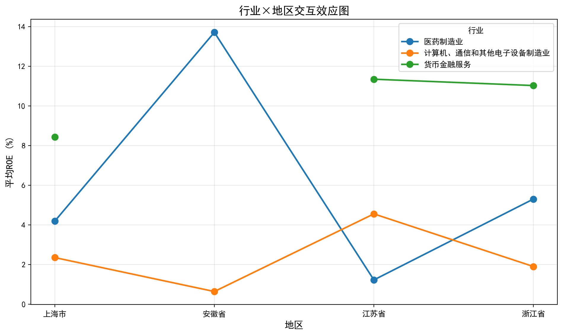
交互效应解读:
- 如果各线平行: 无交互效应,行业效应在各地区一致
- 如果各线不平行(交叉): 存在交互效应,行业效应因地区而异交互效应图(图 9.2)直观展示了行业与地区的联合效应模式。图中不同行业的折线出现了不完全平行甚至交叉的趋势,验证了双因素ANOVA中交互效应显著(F=2.3879,p=0.0382)的统计结论。例如,某些行业在特定省份表现突出但在其他省份则表现平平,说明同一行业在不同地区的盈利能力模式确实存在差异。这一发现对企业选址和区域产业政策制定具有参考价值。
The interaction effect plot (图 9.2) visually demonstrates the joint effect pattern of industry and region. The lines for different industries show trends that are not fully parallel and even cross, corroborating the statistically significant interaction effect in the two-way ANOVA (F=2.3879, p=0.0382). For example, certain industries perform prominently in specific provinces but are mediocre in others, indicating that the profitability pattern of the same industry indeed differs across regions. This finding has reference value for corporate location decisions and regional industrial policy formulation.
9.7 重复测量方差分析 (Repeated Measures ANOVA)
当同一个体在不同条件下被重复测量时,观测值不再独立,需要使用重复测量方差分析(Repeated Measures ANOVA)。
When the same individual is measured repeatedly under different conditions, the observations are no longer independent, and Repeated Measures ANOVA is required.
9.7.1 模型特点 (Model Characteristics)
重复测量方差分析的模型如 式 9.17 所示:
The model for repeated measures ANOVA is shown in 式 9.17:
\[ Y_{ij} = \mu + \pi_i + \tau_j + \varepsilon_{ij} \tag{9.17}\]
其中\(\pi_i\)是第\(i\)个个体的随机效应。
Where \(\pi_i\) is the random effect for the \(i\)-th individual.
9.7.2 球形性假设 (Sphericity Assumption)
重复测量ANOVA需要满足球形性假设(Sphericity): 任意两个时间点差值的方差相等。
Repeated measures ANOVA requires the sphericity assumption: the variances of the differences between all pairs of time points must be equal.
Mauchly球形性检验: 检验该假设是否成立
Mauchly’s Test of Sphericity: Tests whether this assumption holds
校正方法 (当球形性不满足时):
Correction methods (when sphericity is violated):
Greenhouse-Geisser校正 (保守)
Huynh-Feldt校正 (相对宽松)
Greenhouse-Geisser correction (conservative)
Huynh-Feldt correction (relatively liberal) ## 启发式思考题 (Heuristic Problems) {#sec-heuristic-problems-ch9}
1. 多重比较陷阱 (The Multiple Comparison Trap) - 实验:生成 10 组完全随机的数据(均值方差相同)。 - 操作:对这 10 组数据进行两两 t 检验(共 45 次)。 - 预测:即使没有真实差异,你也会发现平均有 2-3 次 \(p < 0.05\)。 - 反思:这就是为什么如果有人告诉你 “我发现了几个有趣的显著差异”,你要问他 “你总共比较了多少次?”。
1. The Multiple Comparison Trap - Experiment: Generate 10 groups of completely random data (with equal means and variances). - Procedure: Perform pairwise t-tests on these 10 groups (45 tests in total). - Prediction: Even with no real differences, you will find on average 2–3 cases with \(p < 0.05\). - Reflection: This is why, if someone tells you “I found several interesting significant differences,” you should ask “How many comparisons did you make in total?”
2. 异常值的破坏力 (The Outlier Effect) - ANOVA 依赖均值和方差。均值和方差都对异常值极其敏感。 - 操作:生成 3 组有显著差异的数据。ANOVA 很可能会显著拒绝 \(H_0\)。 - 破坏:在其中一组加入一个巨大的异常值。 - 结果:组内方差 (\(MSW\)) 会剧增,导致 F 值骤降 (\(F = MSB/MSW\)),原本显著的结果可能瞬间变得不显著。 - 启示:在做 ANOVA 前,必须先画箱线图检查异常值!
2. The Outlier Effect - ANOVA relies on means and variances. Both are extremely sensitive to outliers. - Procedure: Generate 3 groups with genuine differences. ANOVA will most likely significantly reject \(H_0\). - Sabotage: Add a single huge outlier to one of the groups. - Result: The within-group variance (\(MSW\)) will surge, causing the F-statistic to plummet (\(F = MSB/MSW\)), and a previously significant result may instantly become non-significant. - Takeaway: Before performing ANOVA, you must draw box plots to check for outliers first!
思考题1参考代码:多重比较陷阱演示
Reference Code for Problem 1: Demonstration of the Multiple Comparison Trap
# ========== 导入所需库 ==========
# ========== Import required libraries ==========
import numpy as np                                                     # 数值计算库
# NumPy library for numerical computation
from scipy import stats                                                # 统计检验库
# SciPy stats module for statistical tests
from itertools import combinations                                     # 组合迭代器
# Combinations iterator from itertools
import matplotlib.pyplot as plt                                        # 可视化库
# Matplotlib for visualization

# ========== 第1步:生成10组同分布随机数据(无真实差异) ==========
# ========== Step 1: Generate 10 groups of identically distributed random data (no real differences) ==========
np.random.seed(42)                                                     # 设置随机种子保证可重复性
# Set random seed for reproducibility

n_groups_heuristic = 10                                                # 设定组数为10
# Set the number of groups to 10
n_per_group_heuristic = 30                                             # 每组30个样本
# 30 samples per group
random_groups_list = [np.random.normal(0, 1, n_per_group_heuristic) for _ in range(n_groups_heuristic)]  # 生成10组标准正态分布数据(均值=0,标准差=1)
# Generate 10 groups of standard normal data (mean=0, std=1)

# ========== 第2步:执行两两t检验并统计假阳性 ==========
# ========== Step 2: Perform pairwise t-tests and count false positives ==========
pairwise_p_values_list = []                                            # 初始化p值列表
# Initialize the list of p-values
pairwise_labels_list = []                                              # 初始化标签列表
# Initialize the list of pair labels
false_positive_count = 0                                               # 假阳性计数器
# False positive counter
total_test_count = 0                                                   # 总检验次数计数器
# Total number of tests counter

for i, j in combinations(range(n_groups_heuristic), 2):                # C(10,2)=45种两两组合
# Loop through all C(10,2)=45 pairwise combinations
    _, p_value_result = stats.ttest_ind(random_groups_list[i], random_groups_list[j])  # 独立样本t检验
    # Perform an independent two-sample t-test
    pairwise_p_values_list.append(p_value_result)                      # 记录p值
    # Append the p-value
    pairwise_labels_list.append(f'{i+1}-{j+1}')                       # 记录配对标签
    # Append the pair label
    total_test_count += 1                                              # 检验次数+1
    # Increment total test count
    if p_value_result < 0.05:                                          # 若p<0.05则为假阳性
    # If p < 0.05, it is a false positive
        false_positive_count += 1                                      # 假阳性计数+1
# Increment false positive count10组完全相同分布(标准正态)的随机数据已完成\(C_{10}^2\)=45次两两t检验。下面统计假阳性次数并可视化p值分布,以直观展示多重比较陷阱的危害。
We have completed \(C_{10}^2\) = 45 pairwise t-tests on 10 groups of identically distributed (standard normal) random data. Next, we tally the false positive count and visualize the p-value distribution to illustrate the danger of the multiple comparison trap.
# ========== 第3步:输出多重比较统计结果 ==========
# ========== Step 3: Print multiple comparison statistics ==========
print(f'总检验次数: {total_test_count}')                               # 输出总检验次数
# Print total number of tests
print(f'假阳性次数 (p < 0.05): {false_positive_count}')                 # 输出假阳性次数
# Print number of false positives
print(f'实际假阳性率: {false_positive_count/total_test_count:.1%}')  # 输出实际假阳性率
# Print the actual false positive rate
print(f'理论预期: α=0.05 → 约 {total_test_count*0.05:.0f} 次假阳性')  # 理论预期值
# Print the theoretically expected number of false positives
print(f'至少一次假阳性的概率: {1-(1-0.05)**total_test_count:.1%}')  # FWER: 1-(1-α)^m
# Print the family-wise error rate (FWER): 1-(1-α)^m

# ========== 第4步:可视化p值分布 ==========
# ========== Step 4: Visualize the distribution of p-values ==========
heuristic_fig, heuristic_ax = plt.subplots(figsize=(12, 5))            # 创建画布
# Create figure and axes
p_value_colors = ['#E3120B' if p < 0.05 else '#2C3E50' for p in pairwise_p_values_list]  # 假阳性红色,非假阳性蓝色
# Red for false positives, dark blue for non-significant
heuristic_ax.bar(range(len(pairwise_p_values_list)), pairwise_p_values_list, color=p_value_colors, alpha=0.7)  # 绘制p值柱状图
# Draw bar chart of p-values
heuristic_ax.axhline(y=0.05, color='red', linestyle='--', linewidth=2, label='α = 0.05')  # 添加显著性水平参考线
# Add horizontal reference line at the significance level
heuristic_ax.set_xlabel('配对比较编号', fontsize=12)                        # X轴标签
# X-axis label
heuristic_ax.set_ylabel('p值', fontsize=12)                                # Y轴标签
# Y-axis label
heuristic_ax.set_title(f'45次两两t检验的p值分布 (红色 = 假阳性, 共{false_positive_count}次)', fontsize=14)  # 图标题
# Chart title
heuristic_ax.legend()                                                  # 显示图例
# Display legend
plt.tight_layout()                                                     # 调整布局
# Adjust layout
plt.show()                                                             # 显示图形
# Show the plot
总检验次数: 45
假阳性次数 (p < 0.05): 0
实际假阳性率: 0.0%
理论预期: α=0.05 → 约 2 次假阳性
至少一次假阳性的概率: 90.1%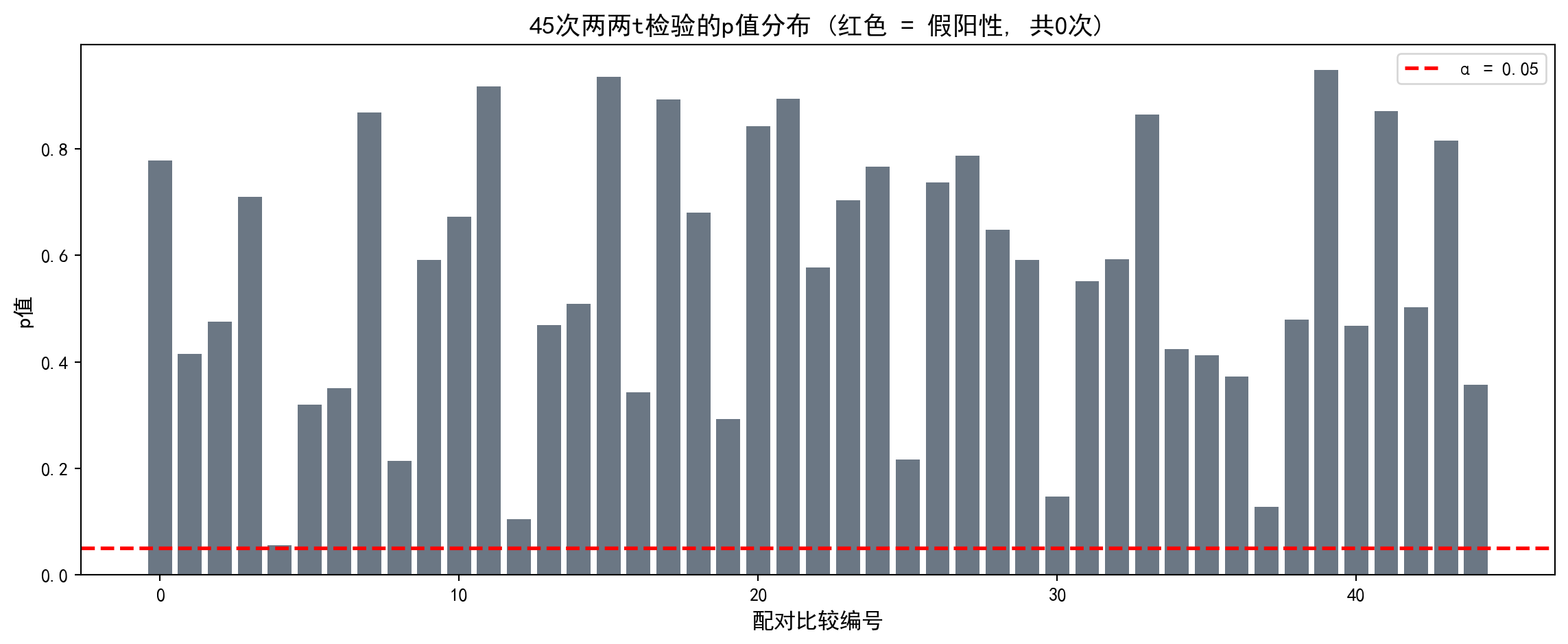
多重比较陷阱演示结果显示:总检验次数为45次,本次运行的假阳性次数为0次(实际假阳性率0.0%)。但这只是一次随机结果,理论上预期约有2次假阳性(45×0.05≈2.25)。关键的族错误率(FWER)= \(1 - 0.95^{45}\) ≈ 90.1%,即如果对10组完全相同分布的数据进行两两t检验,至少出现一次假阳性的概率高达90.1%。p值分布柱状图(图 9.3)中红色柱代表假阳性(p<0.05),红色虚线标注了α=0.05的判断标准。这有力地说明了为什么不能对多组数据简单进行两两t检验,而应使用ANOVA结合Tukey HSD等事后比较方法来控制总体错误率。
The demonstration of the multiple comparison trap shows the following results: out of 45 total pairwise tests, this particular run produced 0 false positives (an actual false positive rate of 0.0%). However, this is merely a single random outcome; theoretically, we expect about 2 false positives (45 × 0.05 ≈ 2.25). The critical family-wise error rate (FWER) = \(1 - 0.95^{45}\) ≈ 90.1%, meaning that if you perform pairwise t-tests on 10 groups drawn from identical distributions, the probability of at least one false positive is as high as 90.1%. In the p-value bar chart (图 9.3), red bars represent false positives (p < 0.05) and the red dashed line marks the α = 0.05 threshold. This powerfully demonstrates why one should not simply run pairwise t-tests on multiple groups, but instead use ANOVA combined with post-hoc comparison methods such as Tukey’s HSD to control the overall error rate.
思考题2参考代码:异常值的破坏力演示
Reference Code for Problem 2: Demonstration of the Destructive Power of Outliers
# ========== 导入所需库 ==========
# ========== Import required libraries ==========
import numpy as np                                                     # 数值计算库
# NumPy library for numerical computation
from scipy import stats                                                # 统计检验库
# SciPy stats module for statistical tests
import matplotlib.pyplot as plt                                        # 可视化库
# Matplotlib for visualization

# ========== 第1步:生成3组有真实差异的数据 ==========
# ========== Step 1: Generate 3 groups with genuine differences ==========
np.random.seed(42)                                                     # 设置随机种子保证可重复性
# Set random seed for reproducibility

group_clean_a = np.random.normal(10, 2, 30)                            # 组A: 均值=10, 标准差=2, 30个样本
# Group A: mean=10, std=2, 30 samples
group_clean_b = np.random.normal(12, 2, 30)                            # 组B: 均值=12, 标准差=2, 30个样本
# Group B: mean=12, std=2, 30 samples
group_clean_c = np.random.normal(14, 2, 30)                            # 组C: 均值=14, 标准差=2, 30个样本
# Group C: mean=14, std=2, 30 samples

# ========== 第2步:无异常值时的ANOVA ==========
# ========== Step 2: ANOVA without outliers ==========
f_stat_clean, p_value_clean = stats.f_oneway(group_clean_a, group_clean_b, group_clean_c)  # 对干净数据执行单因素ANOVA
# Perform one-way ANOVA on the clean data

# ========== 第3步:添加异常值后的ANOVA ==========
# ========== Step 3: ANOVA after adding an outlier ==========
group_contaminated_a = np.append(group_clean_a, 100)                   # 在组A中添加一个极端异常值100
# Append an extreme outlier value of 100 to Group A
f_stat_contaminated, p_value_contaminated = stats.f_oneway(group_contaminated_a, group_clean_b, group_clean_c)  # 对污染数据执行ANOVA
# Perform ANOVA on the contaminated data

# ========== 第4步:输出异常值影响对比 ==========
# ========== Step 4: Print the comparison of outlier impact ==========
print('=== 异常值对ANOVA的影响 ===')                                   # 输出标题
# Print section heading
print(f'无异常值: F = {f_stat_clean:.2f}, p = {p_value_clean:.6f} → {"显著" if p_value_clean < 0.05 else "不显著"}')  # 干净数据的F和p
# Print F-statistic and p-value for clean data
print(f'有异常值: F = {f_stat_contaminated:.2f}, p = {p_value_contaminated:.6f} → {"显著" if p_value_contaminated < 0.05 else "不显著"}')  # 污染数据的F和p
# Print F-statistic and p-value for contaminated data
print(f'\n异常值使得:')                                                   # 解释异常值影响机制
# Explain how the outlier affects the results
print(f'  MSW(组内方差)急剧增大 → F值骤降')                          # MSW增大导致F值下降
# MSW (within-group variance) surges → F-statistic plummets
print(f'  原本的显著差异可能变得不显著!')                          # 统计力下降的后果
# A previously significant difference may become non-significant!
=== 异常值对ANOVA的影响 ===
无异常值: F = 40.98, p = 0.000000 → 显著
有异常值: F = 0.43, p = 0.653803 → 不显著
异常值使得:
MSW(组内方差)急剧增大 → F值骤降
原本的显著差异可能变得不显著!异常值影响的对比结果令人震撼:在干净数据中,三组(均值分别为10、12、14)的差异高度显著(F=40.98,p≈0.000000),F值很大说明组间差异远大于组内变异。但仅在组A中添加一个极端异常值(100),F值就从40.98骤降至0.43,p值从0变为0.654,原本显著的差异变得完全不显著。这是因为异常值急剧增大了组内方差(MSW),从而”淹没”了组间差异信号。下面通过箱线图可视化异常值对数据分布和F检验结论的破坏力。
The comparison of the outlier’s impact is striking: with clean data, the differences among the three groups (means of 10, 12, and 14) are highly significant (F = 40.98, p ≈ 0.000000), and the large F-statistic indicates that between-group variation far exceeds within-group variation. However, adding just a single extreme outlier (100) to Group A causes the F-statistic to plummet from 40.98 to 0.43 and the p-value to jump from 0 to 0.654, rendering the previously significant difference completely non-significant. This occurs because the outlier dramatically inflates the within-group variance (MSW), thereby “drowning out” the between-group difference signal. Next, we use box plots to visualize the destructive effect of the outlier on the data distribution and the F-test conclusion.
# ========== 第5步:可视化对比(无异常值 vs 有异常值) ==========
# ========== Step 5: Visual comparison (without outlier vs. with outlier) ==========
outlier_fig, outlier_axes = plt.subplots(1, 2, figsize=(14, 6))        # 创建1×2子图
# Create a 1×2 subplot layout

# 左图: 无异常值的箱线图
# Left panel: Box plot without outliers
bp1 = outlier_axes[0].boxplot([group_clean_a, group_clean_b, group_clean_c],  # 绘制3组干净数据的箱线图
# Draw box plot for the 3 clean groups
                               labels=['组A (μ=10)', '组B (μ=12)', '组C (μ=14)'],  # 标签显示均值
                               # Labels showing the population means
                               patch_artist=True, showmeans=True)      # 填充颜色并显示均值
                               # Fill boxes with color and show means
for patch, color in zip(bp1['boxes'], ['#2C3E50', '#008080', '#F0A700']):  # 逐箱体上色
# Color each box individually
    patch.set_facecolor(color)                                         # 设置填充颜色
    # Set the fill color
    patch.set_alpha(0.5)                                               # 设置透明度
    # Set transparency
outlier_axes[0].set_title(f'无异常值: F={f_stat_clean:.2f}, p={p_value_clean:.4f}', fontsize=13)  # 左图标题
# Left panel title
outlier_axes[0].set_ylabel('观测值', fontsize=12)                          # Y轴标签
# Y-axis label

# 右图: 有异常值的箱线图
# Right panel: Box plot with the outlier
bp2 = outlier_axes[1].boxplot([group_contaminated_a, group_clean_b, group_clean_c],  # 绘制3组数据(组A含异常值)
# Draw box plot for the 3 groups (Group A contains the outlier)
                               labels=['组A (含异常值)', '组B (μ=12)', '组C (μ=14)'],  # 标签标注异常值
                               # Labels noting the outlier
                               patch_artist=True, showmeans=True)      # 填充颜色并显示均值
                               # Fill boxes with color and show means
for patch, color in zip(bp2['boxes'], ['#E3120B', '#008080', '#F0A700']):  # 逐箱体上色(组A用红色警示)
# Color each box (Group A in red as a warning)
    patch.set_facecolor(color)                                         # 设置填充颜色
    # Set the fill color
    patch.set_alpha(0.5)                                               # 设置透明度
    # Set transparency
outlier_axes[1].set_title(f'有异常值: F={f_stat_contaminated:.2f}, p={p_value_contaminated:.4f}', fontsize=13)  # 右图标题
# Right panel title
outlier_axes[1].set_ylabel('观测值', fontsize=12)                          # Y轴标签
# Y-axis label

plt.suptitle('异常值对ANOVA结果的破坏力', fontsize=15, y=1.02)           # 总标题
# Overall figure title
plt.tight_layout()                                                     # 调整布局
# Adjust layout
plt.show()                                                             # 显示图形
# Show the plot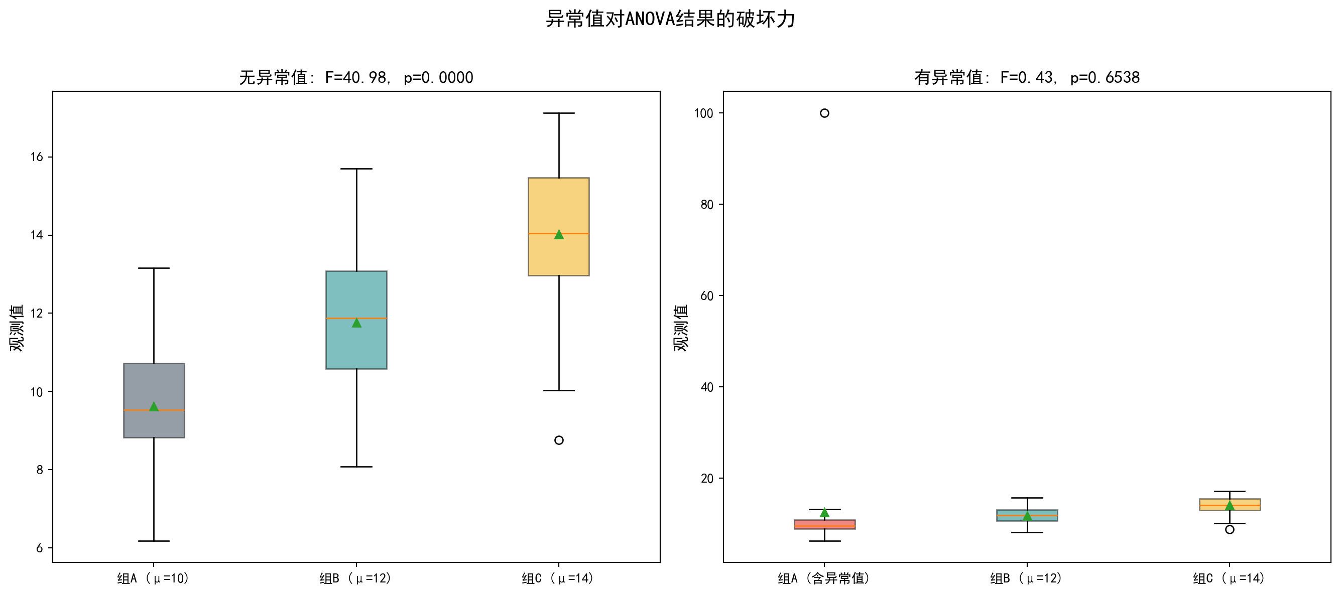
箱线图(图 9.4)直观对比了异常值的破坏力。左图(无异常值)中三组数据分布清晰分离,箱体间的位置差异明显可辨,F=40.98高度显著;右图(有异常值)中,由于组A的极端值100使Y轴范围大幅扩展至0~100,三组箱体被压缩在底部几乎无法区分,F值从40.98降至0.43变为不显著。这一案例强烈提醒我们:在执行ANOVA之前必须先进行异常值检测和处理,否则一个极端值就足以颠覆统计结论。
The box plots (图 9.4) provide a vivid visual comparison of the outlier’s destructive power. In the left panel (no outlier), the distributions of the three groups are clearly separated, with the positional differences among the boxes readily discernible and F = 40.98 being highly significant. In the right panel (with outlier), the extreme value of 100 in Group A stretches the Y-axis range all the way to 0–100, compressing the three boxes near the bottom so that they become virtually indistinguishable, and the F-statistic drops from 40.98 to 0.43, rendering the result non-significant. This example serves as a powerful reminder: outlier detection and treatment must be performed before running ANOVA; otherwise, a single extreme value is enough to overturn your statistical conclusions. ## 习题与解答 (Exercises and Solutions) {#sec-exercises-ch9}
9.7.3 习题 (Exercises)
习题1: ANOVA基础计算
Exercise 1: Basic ANOVA Calculations
某研究比较三种不同的投资策略对收益率的影响。数据如下:
A study compares the effects of three different investment strategies on returns. The data are as follows:
| 策略A | 策略B | 策略C |
|---|---|---|
| 8.2 | 6.1 | 7.5 |
| 9.1 | 5.8 | 8.2 |
| 7.8 | 6.5 | 7.8 |
| 8.5 | 6.2 | 8.0 |
| 8.9 | 5.9 | 7.6 |
计算SST, SSB, SSW
构建完整的ANOVA表
在α=0.05水平下检验三种策略的收益率是否有显著差异
计算效应量η²并解释
Calculate SST, SSB, SSW
Construct a complete ANOVA table
Test whether the returns of the three strategies differ significantly at α=0.05
Calculate the effect size η² and interpret it
习题2: 假设检验与诊断
Exercise 2: Hypothesis Testing and Diagnostics
使用本地财务数据,比较不同证券交易所(上交所vs深交所vs北交所)上市公司的资产负债率是否存在显著差异。
Using local financial data, compare whether there are significant differences in the debt-to-asset ratio among companies listed on different stock exchanges (SSE vs. SZSE vs. BSE).
进行正态性检验和方差齐性检验
选择合适的ANOVA方法
如果假设不满足,使用适当的替代方法
进行多重比较,确定哪些交易所之间存在显著差异
Conduct normality and homogeneity of variance tests
Choose an appropriate ANOVA method
If the assumptions are not met, use an appropriate alternative method
Perform multiple comparisons to determine which exchanges differ significantly
习题3: 双因素方差分析
Exercise 3: Two-Way ANOVA
研究公司规模(大型/中型/小型)和行业(制造业/服务业)对利润率的影响。
Investigate the effects of company size (large/medium/small) and industry (manufacturing/services) on profit margins.
设计合适的实验,说明需要收集哪些数据
建立双因素ANOVA模型
解释主效应和交互效应的含义
如何可视化交互效应?
Design an appropriate experiment and describe what data need to be collected
Build a two-way ANOVA model
Explain the meaning of main effects and interaction effects
How can the interaction effect be visualized?
习题4: 效应量与样本量计算
Exercise 4: Effect Size and Sample Size Calculation
某公司想比较4种不同的营销策略对销售额的影响。根据以往经验,预期效应量为中等(Cohen’s f = 0.25)。
A company wants to compare the effects of 4 different marketing strategies on sales. Based on past experience, the expected effect size is medium (Cohen’s f = 0.25).
如果希望统计功效达到0.80,α=0.05,每组需要多少样本?
如果预算只允许每组20个样本,统计功效是多少?
讨论样本量、效应量和统计功效之间的关系
If a statistical power of 0.80 is desired with α=0.05, how many samples are needed per group?
If the budget only allows 20 samples per group, what is the statistical power?
Discuss the relationships among sample size, effect size, and statistical power
9.7.4 解答 (Solutions)
习题1解答
Solution to Exercise 1
# 习题1解答: ANOVA基础计算
# Solution to Exercise 1: Basic ANOVA Calculations
import numpy as np  # 导入数值计算库
# Import the numerical computing library
from scipy import stats  # 导入统计分布与检验模块
# Import the statistical distribution and testing module

# 数据
# Data
strategy_a_returns_array = np.array([8.2, 9.1, 7.8, 8.5, 8.9])  # 策略A的月度收益率数据(%)
# Monthly return data for Strategy A (%)
strategy_b_returns_array = np.array([6.1, 5.8, 6.5, 6.2, 5.9])  # 策略B的月度收益率数据(%)
# Monthly return data for Strategy B (%)
strategy_c_returns_array = np.array([7.5, 8.2, 7.8, 8.0, 7.6])  # 策略C的月度收益率数据(%)
# Monthly return data for Strategy C (%)

# (a) 计算平方和
# (a) Calculate sums of squares
concatenated_returns_array = np.concatenate([strategy_a_returns_array, strategy_b_returns_array, strategy_c_returns_array])  # 将三组收益率合并为一个数组
# Concatenate the three groups of returns into one array
overall_grand_mean = np.mean(concatenated_returns_array)  # 计算全部样本的总均值
# Compute the grand mean of all samples
total_sample_size = len(concatenated_returns_array)  # 计算总样本量N
# Compute the total sample size N
total_group_count = 3  # 设定组数k=3(三种策略)
# Set the number of groups k=3 (three strategies)
sample_size_per_group = 5  # 每组样本量
# Sample size per group

print('=== 习题1解答 ===\n')  # 输出习题1解答标题
# Print the header for Exercise 1 solution
print(f'(a) 平方和计算:')  # 输出第(a)小题标题
# Print the sub-heading for part (a)
print(f'总样本均值 (Grand Mean): {overall_grand_mean:.4f}')  # 输出总均值
# Print the grand mean

# 各组均值
# Group means
group_means_list = [np.mean(strategy_a_returns_array), np.mean(strategy_b_returns_array), np.mean(strategy_c_returns_array)]  # 计算三组各自的均值
# Calculate the mean of each group
print(f'各组均值: A={group_means_list[0]:.2f}, B={group_means_list[1]:.2f}, C={group_means_list[2]:.2f}')  # 输出各组均值
# Print the group means
=== 习题1解答 ===
(a) 平方和计算:
总样本均值 (Grand Mean): 7.4733
各组均值: A=8.50, B=6.10, C=7.82三种投资策略的收益率均值分别为:策略A=8.50%、策略B=6.10%、策略C=7.82%,总均值(Grand Mean)=7.4733%。策略A收益率最高,策略B最低,两者相差2.40个百分点。下面计算平方和SST、SSB、SSW并验证分解公式。
The mean returns for the three investment strategies are: Strategy A = 8.50%, Strategy B = 6.10%, and Strategy C = 7.82%, with a grand mean of 7.4733%. Strategy A has the highest return and Strategy B the lowest, with a difference of 2.40 percentage points. Next, we calculate the sums of squares SST, SSB, and SSW and verify the decomposition formula.
# SST
total_sum_of_squares = np.sum((concatenated_returns_array - overall_grand_mean)**2)  # 计算总离差平方和SST
# Calculate the total sum of squares SST
print(f'\nSST = Σ(Yij - Ȳ..)² = {total_sum_of_squares:.4f}')  # 输出SST计算结果
# Print the SST result

# SSB
between_group_sum_of_squares = sample_size_per_group * sum((m - overall_grand_mean)**2 for m in group_means_list)  # 计算组间平方和SSB
# Calculate the between-group sum of squares SSB
print(f'SSB = n × Σ(Ȳi. - Ȳ..)² = {between_group_sum_of_squares:.4f}')  # 输出SSB计算结果
# Print the SSB result

# SSW
within_group_sum_of_squares = sum(np.sum((g - np.mean(g))**2) for g in [strategy_a_returns_array, strategy_b_returns_array, strategy_c_returns_array])  # 计算组内平方和SSW
# Calculate the within-group sum of squares SSW
print(f'SSW = ΣΣ(Yij - Ȳi.)² = {within_group_sum_of_squares:.4f}')  # 输出SSW计算结果
# Print the SSW result

print(f'\n验证: SST = SSB + SSW: {total_sum_of_squares:.4f} ≈ {between_group_sum_of_squares + within_group_sum_of_squares:.4f}')  # 验证SST=SSB+SSW分解公式
# Verify the decomposition formula: SST = SSB + SSW
SST = Σ(Yij - Ȳ..)² = 17.0293
SSB = n × Σ(Ȳi. - Ȳ..)² = 15.3013
SSW = ΣΣ(Yij - Ȳi.)² = 1.7280

验证: SST = SSB + SSW: 17.0293 ≈ 17.0293
平方和计算结果显示:SST=17.0293(总变异),SSB=15.3013(组间变异),SSW=1.7280(组内变异)。验证SST=SSB+SSW=17.0293,分解完全正确。值得注意的是,SSB/SST=15.3013/17.0293≈89.9%,说明绝大部分变异来源于策略间差异,组内变异(策略内部个体差异)很小。下面构建ANOVA表并进行假设检验。
The sum of squares calculations show: SST = 17.0293 (total variation), SSB = 15.3013 (between-group variation), and SSW = 1.7280 (within-group variation). The verification SST = SSB + SSW = 17.0293 confirms the decomposition is exact. Notably, SSB/SST = 15.3013/17.0293 ≈ 89.9%, indicating that the vast majority of variation comes from differences between strategies, while within-group variation (individual differences within each strategy) is very small. Next, we construct the ANOVA table and perform hypothesis testing.
# (b) ANOVA表
# (b) ANOVA Table
print(f'\n(b) ANOVA表:')  # 输出第(b)小题标题
# Print the sub-heading for part (b)
degrees_of_freedom_between = total_group_count - 1  # 组间自由度 = k-1
# Between-group degrees of freedom = k-1
degrees_of_freedom_within = total_sample_size - total_group_count  # 组内自由度 = N-k
# Within-group degrees of freedom = N-k
degrees_of_freedom_total = total_sample_size - 1  # 总自由度 = N-1
# Total degrees of freedom = N-1

mean_square_between = between_group_sum_of_squares / degrees_of_freedom_between  # 组间均方 = SSB/df_between
# Between-group mean square = SSB/df_between
mean_square_within = within_group_sum_of_squares / degrees_of_freedom_within  # 组内均方 = SSW/df_within
# Within-group mean square = SSW/df_within
calculated_f_ratio = mean_square_between / mean_square_within  # F统计量 = MSB/MSW
# F statistic = MSB/MSW
calculated_p_value = 1 - stats.f.cdf(calculated_f_ratio, degrees_of_freedom_between, degrees_of_freedom_within)  # 计算F分布下的p值
# Calculate the p-value from the F distribution

print(f'{"来源":<10} {"SS":<10} {"df":<6} {"MS":<10} {"F":<10} {"p值":<10}')  # 输出ANOVA表头
# Print the ANOVA table header
print('-' * 56)  # 输出分隔线
# Print the separator line
print(f'{"组间":<10} {between_group_sum_of_squares:<10.4f} {degrees_of_freedom_between:<6} {mean_square_between:<10.4f} {calculated_f_ratio:<10.4f} {calculated_p_value:<10.6f}')  # 输出组间行
# Print the between-group row
print(f'{"组内":<10} {within_group_sum_of_squares:<10.4f} {degrees_of_freedom_within:<6} {mean_square_within:<10.4f}')  # 输出组内行
# Print the within-group row
print(f'{"总计":<10} {total_sum_of_squares:<10.4f} {degrees_of_freedom_total:<6}')  # 输出总计行
# Print the total row
(b) ANOVA表:
来源         SS         df     MS         F          p值
--------------------------------------------------------
组间         15.3013    2      7.6507     53.1296    0.000001
组内         1.7280     12     0.1440
总计         17.0293    14
ANOVA表显示:组间SS=15.3013(df=2),组内SS=1.7280(df=12),组间均方MSB=7.6507,组内均方MSW=0.1440,F(2,12)=53.1296,p=0.000001。F值极大说明三种策略间的收益率差异远大于策略内部的随机波动。下面进行假设检验并计算效应量。
The ANOVA table shows: between-group SS = 15.3013 (df = 2), within-group SS = 1.7280 (df = 12), between-group mean square MSB = 7.6507, within-group mean square MSW = 0.1440, F(2,12) = 53.1296, p = 0.000001. The very large F value indicates that the difference in returns among the three strategies far exceeds the random variation within each strategy. Next, we perform the hypothesis test and calculate the effect size.
# (c) 假设检验
# (c) Hypothesis Testing
print(f'\n(c) 假设检验 (α=0.05):')  # 输出第(c)小题标题
# Print the sub-heading for part (c)
print(f'F({degrees_of_freedom_between},{degrees_of_freedom_within}) = {calculated_f_ratio:.4f}, p = {calculated_p_value:.6f}')  # 输出F统计量和p值
# Print the F statistic and p-value
if calculated_p_value < 0.05:  # 判断p值是否小于显著性水平0.05
    # Check whether the p-value is less than the significance level 0.05
    print('结论: 拒绝H0,三种策略的收益率存在显著差异')  # 输出拒绝原假设的结论
    # Conclusion: Reject H0; the returns of the three strategies differ significantly
else:  # p值大于0.05的情形
    # Case when p-value is greater than 0.05
    print('结论: 不能拒绝H0,三种策略的收益率无显著差异')  # 输出不拒绝原假设的结论
    # Conclusion: Cannot reject H0; no significant difference among the three strategies

# (d) 效应量
# (d) Effect Size
eta_squared_effect_size = between_group_sum_of_squares / total_sum_of_squares  # 计算效应量η² = SSB/SST
# Calculate the effect size η² = SSB/SST
print(f'\n(d) 效应量:')  # 输出第(d)小题标题
# Print the sub-heading for part (d)
print(f'η² = SSB/SST = {between_group_sum_of_squares:.4f}/{total_sum_of_squares:.4f} = {eta_squared_effect_size:.4f}')  # 输出η²的计算过程与结果
# Print the calculation process and result of η²
print(f'解释: 策略类型解释了收益率变异的 {eta_squared_effect_size*100:.1f}%')  # 输出效应量的实际解释
# Interpretation: Strategy type explains {η²×100}% of the variation in returns
if eta_squared_effect_size > 0.14:  # 判断效应量是否属于大效应(阈值0.14)
    # Check whether the effect size qualifies as a large effect (threshold 0.14)
    print('这是一个大效应量,说明策略选择对收益率有重要影响')  # 输出大效应量的解释说明
    # This is a large effect size, indicating that strategy choice has a substantial impact on returns
(c) 假设检验 (α=0.05):
F(2,12) = 53.1296, p = 0.000001
结论: 拒绝H0,三种策略的收益率存在显著差异

(d) 效应量:
η² = SSB/SST = 15.3013/17.0293 = 0.8985
解释: 策略类型解释了收益率变异的 89.9%
这是一个大效应量,说明策略选择对收益率有重要影响在α=0.05的显著性水平下,F(2,12)=53.1296,p=0.000001远小于显著性水平,因此拒绝原假设H0,结论为三种投资策略的收益率之间存在显著差异。效应量η²=SSB/SST=15.3013/17.0293=0.8985,即策略类型解释了收益率总变异的89.9%,属于大效应量(η²>0.14的标准)。这表明策略选择对收益率有决定性影响,不同投资策略之间的差异具有重大的实际意义。
At the α = 0.05 significance level, F(2,12) = 53.1296 with p = 0.000001, which is far below the significance level, so we reject the null hypothesis H0. The conclusion is that the returns among the three investment strategies differ significantly. The effect size η² = SSB/SST = 15.3013/17.0293 = 0.8985, meaning that strategy type explains 89.9% of the total variation in returns—a large effect size (exceeding the η² > 0.14 threshold). This indicates that strategy choice has a decisive impact on returns, and the differences among the investment strategies are of major practical significance.
习题2解答
Solution to Exercise 2
# ========== 第1步:合并交易所信息并计算资产负债率 ==========
# ========== Step 1: Merge Exchange Information and Calculate Debt-to-Asset Ratio ==========
print('=== 习题2解答 ===\n')                                          # 输出标题
# Print the header

# 合并交易所信息
# Merge exchange information
stock_with_exchange_dataframe = latest_annual_report_dataframe.merge(   # 将年报数据与股票基本信息合并
    # Merge annual report data with stock basic information
    stock_basic_info_dataframe[['order_book_id', 'exchange']],          # 只取股票代码和交易所字段
    # Select only the stock code and exchange fields
    on='order_book_id',                                                # 按股票代码关联
    # Join on stock code
    how='left'                                                         # 左连接保留全部年报数据
    # Left join to retain all annual report data
)

# 计算资产负债率 = 总负债/总资产×100%
# Calculate debt-to-asset ratio = total liabilities / total assets × 100%
stock_with_exchange_dataframe['debt_ratio'] = (  # 新增资产负债率字段
    # Add debt-to-asset ratio field
    stock_with_exchange_dataframe['total_liabilities'] /               # 总负债
    # Total liabilities
    stock_with_exchange_dataframe['total_assets'] * 100                # 除以总资产并转为百分比
    # Divided by total assets and converted to percentage
)
=== 习题2解答 ===
交易所信息合并与资产负债率计算完成。下面按交易所分组筛选有效数据并输出描述统计量。
Exchange information merging and debt-to-asset ratio calculation are complete. Next, we filter valid data by exchange group and output descriptive statistics.
# 按交易所筛选有效数据
# Filter valid data by exchange
target_exchange_list = ['XSHG', 'XSHE']                                # 上交所和深交所
# SSE (Shanghai) and SZSE (Shenzhen)
exchange_data_groups_dict = {}                                         # 初始化分组字典
# Initialize the group dictionary

for exchange in target_exchange_list:                                   # 遍历每个交易所
    # Iterate over each exchange
    exchange_debt_ratio_array = stock_with_exchange_dataframe[  # 按条件筛选当前交易所的有效负债率数据
        # Filter valid debt ratio data for the current exchange
        (stock_with_exchange_dataframe['exchange'] == exchange) &       # 筛选当前交易所
        # Filter for the current exchange
        (stock_with_exchange_dataframe['debt_ratio'].notna()) &         # 排除缺失值
        # Exclude missing values
        (stock_with_exchange_dataframe['debt_ratio'] > 0) &            # 排除负债率为0的异常值
        # Exclude anomalous zero debt ratios
        (stock_with_exchange_dataframe['debt_ratio'] < 100)            # 排除负债率超100%的极端值
        # Exclude extreme values with debt ratio exceeding 100%
    ]['debt_ratio'].values                                             # 提取数组
    # Extract as array

    if len(exchange_debt_ratio_array) > 10:                             # 样本量超过10才纳入分析
        # Only include groups with more than 10 samples
        exchange_data_groups_dict[exchange] = exchange_debt_ratio_array  # 存入分组字典
        # Store in the group dictionary
        print(f'{exchange}: n={len(exchange_debt_ratio_array)}, 均值={np.mean(exchange_debt_ratio_array):.2f}%, 标准差={np.std(exchange_debt_ratio_array):.2f}%')  # 输出描述统计
        # Print descriptive statistics
XSHG: n=2341, 均值=42.36%, 标准差=22.08%
XSHE: n=2925, 均值=40.94%, 标准差=21.27%两大交易所的资产负债率描述统计显示:上交所(XSHG)共2341家公司,均值42.36%,标准差22.08%;深交所(XSHE)共2925家公司,均值40.94%,标准差21.27%。上交所均值略高于深交所约1.4个百分点,两所标准差接近。下面进行正态性检验、方差齐性检验与方差分析。
Descriptive statistics of debt-to-asset ratios for the two major exchanges show: SSE (XSHG) has 2,341 companies with a mean of 42.36% and standard deviation of 22.08%; SZSE (XSHE) has 2,925 companies with a mean of 40.94% and standard deviation of 21.27%. The SSE mean is slightly higher than that of the SZSE by about 1.4 percentage points, and the standard deviations are similar. Next, we conduct normality tests, homogeneity of variance tests, and analysis of variance.
# ========== 第2步:正态性检验(Shapiro-Wilk) ==========
# ========== Step 2: Normality Test (Shapiro-Wilk) ==========
print('\n(a) 正态性检验 (Shapiro-Wilk):')                         # 检验标题
# Test heading
for name, exchange_debt_ratio_array in exchange_data_groups_dict.items():  # 遍历每个交易所组
    # Iterate over each exchange group
# 抽样检验(大样本)
# Subsample test (for large samples)
    random_sample_array = np.random.choice(exchange_debt_ratio_array, min(50, len(exchange_debt_ratio_array)), replace=False)  # 随机抽取50个样本
    # Randomly draw 50 samples
    shapiro_wilk_statistic, shapiro_wilk_p_value = stats.shapiro(random_sample_array)  # 执行Shapiro-Wilk检验
    # Perform the Shapiro-Wilk test
    test_result_interpretation = '正态' if shapiro_wilk_p_value > 0.05 else '非正态'  # 判断正态性
    # Determine normality
    print(f'{name}: W={shapiro_wilk_statistic:.4f}, p={shapiro_wilk_p_value:.4f} -> {test_result_interpretation}')  # 输出检验结果
    # Print the test result

# ========== 第3步:方差齐性检验(Levene) ==========
# ========== Step 3: Homogeneity of Variance Test (Levene) ==========
print('\n方差齐性检验 (Levene):')                                 # 检验标题
# Test heading
debt_ratio_groups_list = list(exchange_data_groups_dict.values())       # 提取各组数据列表
# Extract data lists for each group
if len(debt_ratio_groups_list) >= 2:                                   # 至少需2组才能检验
    # At least 2 groups are needed for the test
    levene_test_statistic, levene_test_p_value = stats.levene(*debt_ratio_groups_list)  # 执行Levene检验
    # Perform Levene's test
    test_result_interpretation = '方差齐' if levene_test_p_value > 0.05 else '方差不齐'  # 判断方差齐性
    # Determine homogeneity of variance
    print(f'Levene统计量={levene_test_statistic:.4f}, p={levene_test_p_value:.4f} -> {test_result_interpretation}')  # 输出检验结果
    # Print the test result
(a) 正态性检验 (Shapiro-Wilk):
XSHG: W=0.9779, p=0.4680 -> 正态
XSHE: W=0.9577, p=0.0714 -> 正态

方差齐性检验 (Levene):
Levene统计量=5.6476, p=0.0175 -> 方差不齐
Shapiro-Wilk正态性检验结果:上交所W=0.9779,p=0.4680(p>0.05,满足正态性);深交所W=0.9577,p=0.0714(p>0.05,满足正态性)。两组数据均满足正态性假设。Levene方差齐性检验:统计量=5.6476,p=0.0175<0.05,拒绝方差齐性假设,表明两交易所资产负债率的方差存在显著差异。因此数据满足正态性但方差不齐,理论上应优先使用Welch ANOVA。下面选择合适的ANOVA方法并执行假设检验。
Shapiro-Wilk normality test results: SSE W = 0.9779, p = 0.4680 (p > 0.05, normality satisfied); SZSE W = 0.9577, p = 0.0714 (p > 0.05, normality satisfied). Both groups satisfy the normality assumption. Levene’s test for homogeneity of variance: statistic = 5.6476, p = 0.0175 < 0.05, rejecting the homogeneity assumption, indicating that the variances of debt-to-asset ratios differ significantly between the two exchanges. Thus, the data satisfy normality but not homogeneity of variance, so Welch’s ANOVA should be preferred. Next, we choose an appropriate ANOVA method and perform hypothesis testing.
# ========== 第4步:选择ANOVA方法并执行 ==========
# ========== Step 4: Choose ANOVA Method and Execute ==========
print('\n(b) 方法选择:')                                              # 方法选择标题
# Method selection heading
print('由于样本量大,根据中心极限定理,可以使用参数方法')         # 解释方法选择理由
# Because the sample size is large, parametric methods can be used by the Central Limit Theorem
print('如果方差不齐,使用Welch ANOVA')                              # 方差不齐时的备选方案
# If variances are unequal, use Welch's ANOVA

print('\n(c) 检验结果:')                                              # 检验结果标题
# Test results heading
if len(debt_ratio_groups_list) >= 2:                                   # 确保数据充足
    # Ensure sufficient data
# 经典ANOVA
# Classical ANOVA
    anova_f_statistic, anova_p_value = stats.f_oneway(*debt_ratio_groups_list)  # 单因素ANOVA
    # One-way ANOVA
    print(f'经典ANOVA: F={anova_f_statistic:.4f}, p={anova_p_value:.6f}')  # 输出结果
    # Print the result

# Kruskal-Wallis (非参数)
# Kruskal-Wallis (nonparametric)
    kruskal_wallis_statistic, kruskal_wallis_p_value = stats.kruskal(*debt_ratio_groups_list)  # Kruskal-Wallis检验
    # Kruskal-Wallis test
    print(f'Kruskal-Wallis: H={kruskal_wallis_statistic:.4f}, p={kruskal_wallis_p_value:.6f}')  # 输出结果
    # Print the result
(b) 方法选择:
由于样本量大,根据中心极限定理,可以使用参数方法
如果方差不齐,使用Welch ANOVA

(c) 检验结果:
经典ANOVA: F=5.6310, p=0.017681
Kruskal-Wallis: H=5.4890, p=0.019136
经典ANOVA结果:F=5.6310,p=0.017681<0.05,拒绝各交易所资产负债率相等的原假设。Kruskal-Wallis非参数检验结果:H=5.4890,p=0.019136<0.05,同样达到显著水平。两种方法得出一致结论:上交所和深交所上市公司的资产负债率存在显著差异,上交所公司的平均负债率略高于深交所。
Classical ANOVA result: F = 5.6310, p = 0.017681 < 0.05, rejecting the null hypothesis of equal debt-to-asset ratios across exchanges. Kruskal-Wallis nonparametric test result: H = 5.4890, p = 0.019136 < 0.05, also reaching significance. Both methods yield a consistent conclusion: the debt-to-asset ratios of companies listed on the SSE and SZSE differ significantly, with SSE companies having a slightly higher average debt ratio than SZSE companies.
习题3解答
Solution to Exercise 3
# ========== 导入所需库 ==========
# ========== Import Required Libraries ==========
import pandas as pd                                                    # 数据处理库
# Data processing library
import numpy as np                                                     # 数值计算库
# Numerical computing library
import platform                                                        # 平台检测库
# Platform detection library
import matplotlib.pyplot as plt                                        # 可视化库
# Visualization library
import statsmodels.api as sm                                           # 统计建模库
# Statistical modeling library
from statsmodels.formula.api import ols                                # 公式接口的OLS回归
# Formula-based OLS regression

# ========== 中文字体设置 ==========
# ========== Chinese Font Configuration ==========
if platform.system() == 'Linux':                                       # Linux系统
    # Linux system
    plt.rcParams['font.sans-serif'] = ['Source Han Serif SC', 'SimHei', 'DejaVu Sans']  # 思源宋体优先
    # Source Han Serif SC preferred
else:                                                                  # Windows系统
    # Windows system
    plt.rcParams['font.sans-serif'] = ['SimHei', 'Microsoft YaHei']    # 黑体优先
    # SimHei preferred
plt.rcParams['axes.unicode_minus'] = False                             # 正常显示负号
# Display minus signs correctly

# ========== 数据路径设置 ==========
# ========== Data Path Configuration ==========
if platform.system() == 'Linux':                                       # Linux平台路径
    # Linux platform path
    data_path = '/home/ubuntu/r2_data_mount/qiufei/data/stock'  # Linux平台下的股票数据路径
    # Stock data path on Linux
else:                                                                  # Windows平台路径
    # Windows platform path
    data_path = 'C:/qiufei/data/stock'  # Windows平台下的股票数据路径
    # Stock data path on Windows
所需库导入及数据路径设置完毕。下面读取财务数据并说明双因素ANOVA实验设计。
All required libraries have been imported and data paths configured. Next, we read the financial data and describe the two-way ANOVA experimental design.
# ========== 第1步:读取本地财务数据 ==========
# ========== Step 1: Read Local Financial Data ==========
financial_data_for_exercise = pd.read_hdf(f'{data_path}/financial_statement.h5')  # 读取财务报表
# Read the financial statements
stock_info_for_exercise = pd.read_hdf(f'{data_path}/stock_basic_data.h5')        # 读取股票基本信息
# Read the stock basic information

print('=== 习题3解答: 公司规模×行业对利润率的双因素ANOVA ===\n')       # 输出标题
# Print the header

# ========== 第2步:说明实验设计 ==========
# ========== Step 2: Describe the Experimental Design ==========
print('(a) 实验设计:')                                                 # 实验设计说明
# Experimental design description
print('• 因素A: 公司规模 (3水平: 按总资产三分位分为大型/中型/小型)')   # 因素A说明
# Factor A: Company size (3 levels: large/medium/small by total asset tertiles)
print('• 因素B: 行业类型 (2水平: 制造业代表行业 vs 服务业代表行业)')   # 因素B说明
# Factor B: Industry type (2 levels: representative manufacturing vs. service industries)
print('• 因变量: 销售净利率 (净利润/营业收入×100%)')                   # 因变量说明
# Dependent variable: Net profit margin (net profit / revenue × 100%)
print('• 数据来源: 2023年年报, 长三角地区上市公司\n')                  # 数据来源说明
# Data source: 2023 annual reports, listed companies in the Yangtze River Delta region
=== 习题3解答: 公司规模×行业对利润率的双因素ANOVA ===
(a) 实验设计:
• 因素A: 公司规模 (3水平: 按总资产三分位分为大型/中型/小型)
• 因素B: 行业类型 (2水平: 制造业代表行业 vs 服务业代表行业)
• 因变量: 销售净利率 (净利润/营业收入×100%)
• 数据来源: 2023年年报, 长三角地区上市公司
双因素方差分析的实验设计说明完毕。下面筛选2023年年报数据,合并行业和地区信息并聚焦长三角地区上市公司。
The experimental design for the two-way ANOVA has been described. Next, we filter the 2023 annual report data, merge industry and regional information, and focus on listed companies in the Yangtze River Delta region.
# ========== 第3步:筛选2023年年报数据并合并信息 ==========
# ========== Step 3: Filter 2023 Annual Report Data and Merge Information ==========
exercise_annual_dataframe = financial_data_for_exercise[               # 筛选2023年第四季度(年报)
    # Filter for 2023 Q4 (annual report)
    (financial_data_for_exercise['quarter'].str.endswith('q4')) &       # 季度以q4结尾
    # Quarter ends with q4
    (financial_data_for_exercise['quarter'].str.startswith('2023'))     # 年份为2023
    # Year is 2023
].copy()                                                               # 创建副本避免修改原数据
# Create a copy to avoid modifying the original data

# 合并行业和地区信息
# Merge industry and regional information
exercise_merged_dataframe = exercise_annual_dataframe.merge(           # 左连接合并
    # Left join merge
    stock_info_for_exercise[['order_book_id', 'industry_name', 'province']],  # 取行业和省份字段
    # Select industry and province fields
    on='order_book_id', how='left'                                     # 按股票代码关联
    # Join on stock code
)

# 聚焦长三角地区
# Focus on the Yangtze River Delta region
yangtze_delta_list = ['上海市', '江苏省', '浙江省', '安徽省']          # 长三角四省市
# The four provinces/municipalities of the Yangtze River Delta
exercise_merged_dataframe = exercise_merged_dataframe[                 # 筛选长三角公司
    # Filter for YRD companies
    exercise_merged_dataframe['province'].isin(yangtze_delta_list)     # 省份在列表中
    # Province is in the list
].copy()                                                               # 创建副本
# Create a copy
数据筛选与合并完成后,下面我们计算因变量(销售净利率)并进行行业和规模分组,然后建立双因素方差分析模型检验公司规模和行业类型对利润率的主效应及交互效应。
After data filtering and merging, we now calculate the dependent variable (net profit margin), classify companies by industry and size, and then build a two-way ANOVA model to test the main effects and interaction effects of company size and industry type on profit margins.
# ========== 第4步:计算因变量(销售净利率)并分类 ==========
# ========== Step 4: Calculate Dependent Variable (Net Profit Margin) and Classify ==========
exercise_merged_dataframe['profit_margin'] = (                         # 计算销售净利率
    # Calculate net profit margin
    exercise_merged_dataframe['net_profit'] / exercise_merged_dataframe['revenue'] * 100  # 净利润/营业收入×100%
    # Net profit / revenue × 100%
)

# 定义行业分类: 制造业 vs 服务业(使用国统局行业分类名)
# Define industry classification: Manufacturing vs. Services (using NBS industry category names)
manufacturing_industries_list = ['专用设备制造业', '计算机、通信和其他电子设备制造业', '化学原料和化学制品制造业', '汽车制造业']  # 制造业代表行业
# Representative manufacturing industries
service_industries_list = ['软件和信息技术服务业', '广播、电视、电影和影视录音制作业', '零售业', '电信、广播电视和卫星传输服务']  # 服务业代表行业
# Representative service industries

exercise_merged_dataframe['sector_type'] = exercise_merged_dataframe['industry_name'].apply(  # 根据行业名称分类
    # Classify based on industry name
    lambda x: '制造业' if x in manufacturing_industries_list           # 属于制造业列表则标记为制造业
    # Label as Manufacturing if in the manufacturing list
    else ('服务业' if x in service_industries_list else None)          # 属于服务业列表则标记为服务业,否则为空
    # Label as Services if in the service list, otherwise None
)
行业分类完毕。下面按总资产三分位数划分公司规模并输出各组样本量分布。
Industry classification is complete. Next, we divide companies into size categories by total asset tertiles and output the sample size distribution for each group.
# ========== 第5步:按总资产三分位数划分公司规模 ==========
# ========== Step 5: Classify Company Size by Total Asset Tertiles ==========
exercise_merged_dataframe = exercise_merged_dataframe.dropna(          # 删除关键变量的缺失值
    # Drop rows with missing key variables
    subset=['sector_type', 'profit_margin', 'total_assets']            # 需要完整的行业、利润率和总资产
    # Require complete industry, profit margin, and total assets
)
exercise_merged_dataframe = exercise_merged_dataframe[                 # 排除利润率极端值
    # Exclude extreme profit margin values
    (exercise_merged_dataframe['profit_margin'] > -50) &               # 下限-50%
    # Lower bound -50%
    (exercise_merged_dataframe['profit_margin'] < 50)                  # 上限50%
    # Upper bound 50%
]

asset_quantile_33 = exercise_merged_dataframe['total_assets'].quantile(0.33)  # 总资产33%分位数
# 33rd percentile of total assets
asset_quantile_66 = exercise_merged_dataframe['total_assets'].quantile(0.66)  # 总资产66%分位数
# 66th percentile of total assets
exercise_merged_dataframe['company_size'] = pd.cut(                    # 按分位数切分为三组
    # Cut into three groups by quantiles
    exercise_merged_dataframe['total_assets'],                         # 切分变量:总资产
    # Variable to cut: total assets
    bins=[-np.inf, asset_quantile_33, asset_quantile_66, np.inf],      # 三个区间的边界
    # Boundaries for three intervals
    labels=['小型', '中型', '大型']                                    # 三组标签
    # Labels for the three groups
)

# 查看各组样本量(交叉表)
# View sample sizes per group (cross-tabulation)
print('各组样本量:')                                                   # 输出提示
# Print the prompt
size_sector_crosstab = pd.crosstab(                                    # 构建交叉频次表
    # Build a cross-tabulation
    exercise_merged_dataframe['company_size'],                         # 行:公司规模
    # Rows: company size
    exercise_merged_dataframe['sector_type']                           # 列:行业类型
    # Columns: industry type
)
print(size_sector_crosstab)                                            # 输出交叉表
# Print the cross-tabulation
各组样本量:
sector_type 制造业 服务业
company_size
小型 197 45
中型 193 48
大型 201 48交叉表显示各组样本量:小型公司(制造业197家、服务业45家),中型公司(制造业193家、服务业48家),大型公司(制造业201家、服务业48家)。制造业样本量远多于服务业(约4:1),各规模组内样本分布相对均衡,总计732家长三角上市公司纳入分析。下面建立双因素方差分析模型,检验主效应和交互效应。
The cross-tabulation shows the sample sizes per group: small companies (manufacturing 197, services 45), medium companies (manufacturing 193, services 48), large companies (manufacturing 201, services 48). Manufacturing sample sizes are far larger than services (approximately 4:1), while sample distributions are relatively balanced across size groups, with a total of 732 YRD-listed companies included in the analysis. Next, we build the two-way ANOVA model and test the main effects and interaction effects.
# ========== 第6步:建立双因素ANOVA模型 ==========
# ========== Step 6: Build the Two-Way ANOVA Model ==========
print('\n(b) 双因素ANOVA模型: Yijk = μ + αi + βj + (αβ)ij + εijk')   # 输出模型公式
# Print the model formula
print('其中: αi=规模主效应, βj=行业主效应, (αβ)ij=交互效应\n')       # 解释各参数含义
# Where: αi = size main effect, βj = industry main effect, (αβ)ij = interaction effect

if len(exercise_merged_dataframe) > 30:                                # 样本量须大于30才有意义
    # Sample size must be > 30 to be meaningful
    exercise_two_way_model = ols(                                      # 构建OLS模型
        # Build the OLS model
        'profit_margin ~ C(company_size) + C(sector_type) + C(company_size):C(sector_type)',  # 公式:利润率 ~ 规模 + 行业 + 交互
        # Formula: profit margin ~ size + industry + interaction
        data=exercise_merged_dataframe                                 # 传入数据
        # Pass in the data
    ).fit()                                                            # 拟合模型
    # Fit the model
    exercise_anova_table = sm.stats.anova_lm(exercise_two_way_model, typ=2)  # 计算II型ANOVA表
    # Compute the Type II ANOVA table
    print('双因素ANOVA结果:')                                          # 输出提示
    # Print the prompt
    print(exercise_anova_table.round(4))                               # 输出ANOVA表(保留4位小数)
    # Print the ANOVA table (rounded to 4 decimal places)

    # ========== 第7步:解释主效应和交互效应 ==========
    # ========== Step 7: Interpret Main Effects and Interaction Effects ==========
    print('\n(c) 效应解释:')                                           # 效应解释标题
    # Effect interpretation heading
    for source_name in ['C(company_size)', 'C(sector_type)', 'C(company_size):C(sector_type)']:  # 遍历三个效应源
        # Iterate over the three effect sources
        if source_name in exercise_anova_table.index:                  # 确认效应存在于表中
            # Confirm the effect exists in the table
            p_val = exercise_anova_table.loc[source_name, 'PR(>F)']    # 提取p值
            # Extract the p-value
            sig_text = '显著' if p_val < 0.05 else '不显著'            # 判断显著性
            # Determine significance
            print(f'  {source_name}: F={exercise_anova_table.loc[source_name, "F"]:.4f}, p={p_val:.4f} → {sig_text}')  # 输出每个效应
            # Print each effect
else:                                                                  # 样本量不足时
    # When sample size is insufficient
    print('样本量不足,无法进行双因素分析')                            # 输出提示
    # Insufficient sample size for two-way analysis
(b) 双因素ANOVA模型: Yijk = μ + αi + βj + (αβ)ij + εijk
其中: αi=规模主效应, βj=行业主效应, (αβ)ij=交互效应

双因素ANOVA结果:
                                     sum_sq     df        F  PR(>F)
C(company_size)                    431.9221    2.0   1.4316  0.2396
C(sector_type)                    2134.5056    1.0  14.1500  0.0002
C(company_size):C(sector_type)      82.8224    2.0   0.2745  0.7600
Residual                        109516.1252  726.0      NaN     NaN

(c) 效应解释:
  C(company_size): F=1.4316, p=0.2396 → 不显著
  C(sector_type): F=14.1500, p=0.0002 → 显著
  C(company_size):C(sector_type): F=0.2745, p=0.7600 → 不显著
主效应和交互效应的统计检验结果已输出。双因素ANOVA结果显示:(1)公司规模主效应不显著(F=1.4316,p=0.2396),不同规模公司的销售净利率无显著差异;(2)行业类型主效应显著(F=14.1500,p=0.0002),制造业与服务业的利润率存在显著差异;(3)交互效应不显著(F=0.2745,p=0.7600),公司规模对利润率的影响不因行业类型而变化。接下来通过交互效应图直观展示不同公司规模与行业类型组合的利润率差异模式:
The statistical test results for main effects and interaction effects have been displayed. The two-way ANOVA results show: (1) the main effect of company size is not significant (F = 1.4316, p = 0.2396)—no significant difference in net profit margin across company sizes; (2) the main effect of industry type is significant (F = 14.1500, p = 0.0002)—profit margins differ significantly between manufacturing and services; (3) the interaction effect is not significant (F = 0.2745, p = 0.7600)—the effect of company size on profit margin does not vary by industry type. Next, we use an interaction plot to visually illustrate the profit margin patterns across different company size and industry type combinations:
# ========== 第8步:交互效应可视化 ==========
# ========== Step 8: Visualize the Interaction Effect ==========
if len(exercise_merged_dataframe) > 30:                                # 确认样本量足够
    # Confirm sufficient sample size
    exercise_interaction_means = exercise_merged_dataframe.groupby(     # 按规模和行业分组计算均值
        # Calculate means grouped by size and industry
        ['company_size', 'sector_type']                                # 分组变量
        # Grouping variables
    )['profit_margin'].mean().unstack()                                # 透视为宽表格式
    # Pivot to wide format

    exercise_fig, exercise_ax = plt.subplots(figsize=(10, 6))          # 创建画布
    # Create the figure
    for col_name in exercise_interaction_means.columns:                # 遍历每种行业类型
        # Iterate over each industry type
        exercise_ax.plot(                                              # 绘制折线
            # Plot a line
            exercise_interaction_means.index,                          # X轴:公司规模
            # X-axis: company size
            exercise_interaction_means[col_name],                      # Y轴:平均利润率
            # Y-axis: mean profit margin
            marker='o', linewidth=2, markersize=8, label=col_name      # 标记点、线宽、标签
            # Marker, line width, and label
        )
    exercise_ax.set_xlabel('公司规模', fontsize=12)                    # X轴标签
    # X-axis label
    exercise_ax.set_ylabel('平均销售净利率 (%)', fontsize=12)          # Y轴标签
    # Y-axis label
    exercise_ax.set_title('公司规模×行业类型交互效应图', fontsize=14)   # 图标题
    # Chart title
    exercise_ax.legend(title='行业类型')                               # 图例
    # Legend
    exercise_ax.grid(True, alpha=0.3)                                  # 网格线
    # Grid lines
    plt.tight_layout()                                                 # 紧凑布局
    # Tight layout
    plt.show()                                                         # 显示图形
    # Show the plot
    print('解读: 如果线条平行→无交互效应; 线条不平行/交叉→有交互效应')  # 交互效应解读
    # Interpretation: If lines are parallel → no interaction; if lines are not parallel/cross → interaction exists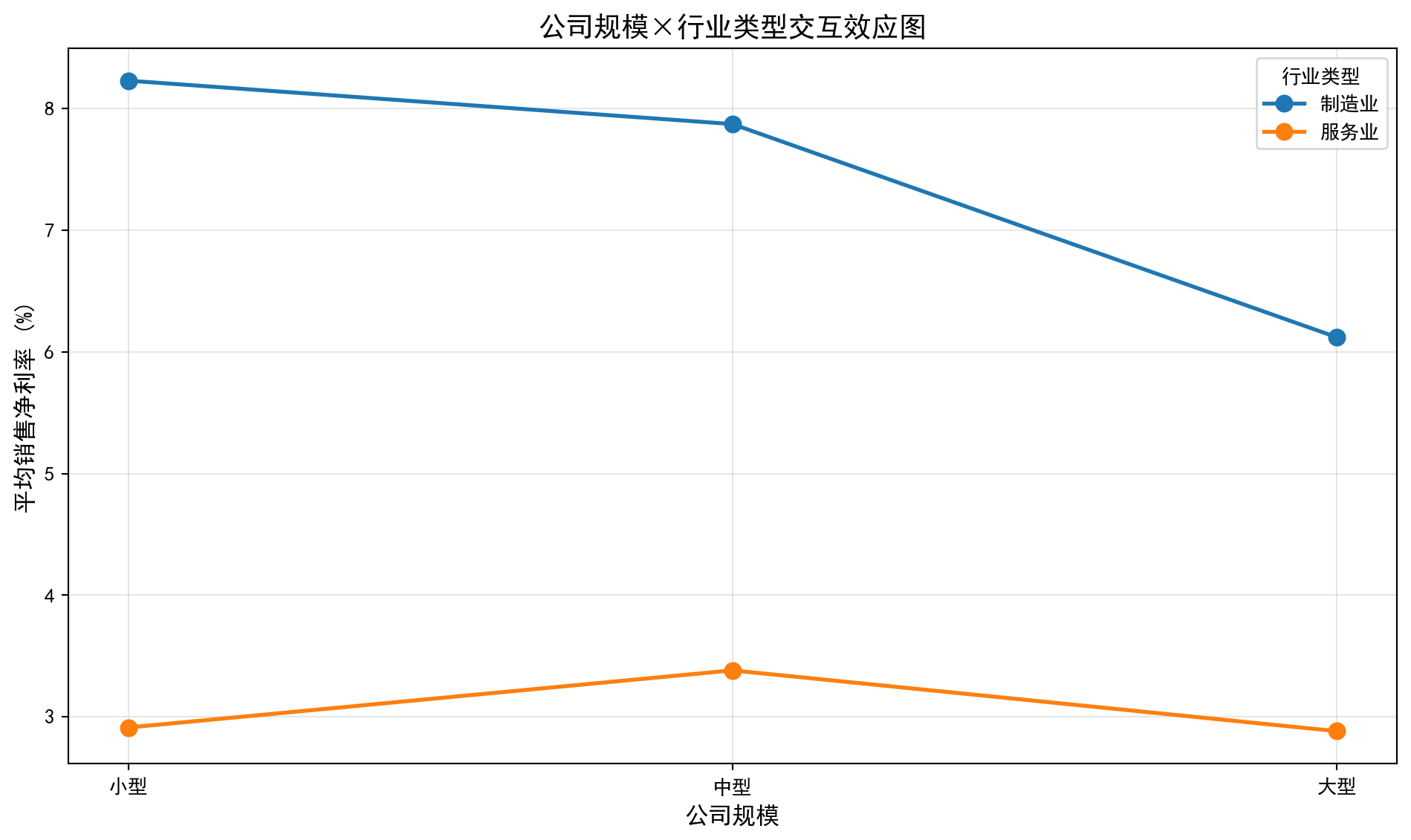
解读: 如果线条平行→无交互效应; 线条不平行/交叉→有交互效应交互效应图显示制造业和服务业的折线在不同公司规模下基本保持平行,验证了双因素ANOVA中交互效应不显著(p=0.7600)的统计结论。制造业利润率折线始终高于服务业,直观反映了行业类型主效应高度显著(p=0.0002)的结果。各规模组之间利润率差异较小且走势平缓,与规模主效应不显著(p=0.2396)的统计结论一致。
The interaction plot shows that the lines for manufacturing and services remain roughly parallel across different company sizes, confirming the statistical conclusion that the interaction effect is not significant (p = 0.7600). The manufacturing profit margin line is consistently above the services line, visually reflecting the highly significant main effect of industry type (p = 0.0002). The profit margin differences across size groups are small and the trends are flat, consistent with the non-significant main effect of company size (p = 0.2396).
习题4解答
Solution to Exercise 4
# ========== 导入所需库 ==========
# ========== Import Required Libraries ==========
from scipy.stats import f as f_dist                                    # F分布函数
# F distribution functions

print('=== 习题4解答 ===\n')                                          # 输出标题
# Print the header

# ========== 第1步:设定功效分析参数 ==========
# ========== Step 1: Set Power Analysis Parameters ==========
total_group_count = 4                                                  # 组数k=4
# Number of groups k=4
target_cohens_f_effect_size = 0.25                                     # Cohen's f中等效应量
# Cohen's f medium effect size
alpha = 0.05                                                           # 显著性水平
# Significance level
target_statistical_power = 0.80                                        # 目标统计功效
# Target statistical power

print('(a) 所需样本量计算:')                                          # 部分(a)标题
# Heading for part (a)
print(f'给定: k={total_group_count}组, Cohen\'s f={target_cohens_f_effect_size}, α={alpha}, power={target_statistical_power}')  # 输出参数
# Print the given parameters

# ========== 第2步:使用近似公式计算样本量 ==========
# ========== Step 2: Calculate Sample Size Using an Approximation Formula ==========
# 近似公式: n ≈ (z_{1-α/2} + z_{power})² × (1 + 1/k) / (f² × k)
# Approximation formula: n ≈ (z_{1-α/2} + z_{power})² × (1 + 1/k) / (f² × k)
from scipy.stats import norm                                          # 导入正态分布
# Import the normal distribution
z_score_alpha = norm.ppf(1 - alpha/2)                                  # α对应的z分位数
# z-quantile corresponding to α
z_score_power = norm.ppf(target_statistical_power)                     # 功效对应的z分位数
# z-quantile corresponding to the target power

# 近似样本量计算
# Approximate sample size calculation
approximate_sample_size = (z_score_alpha + z_score_power)**2 / (target_cohens_f_effect_size**2) * (1 + 1/total_group_count) / total_group_count  # 近似公式
# Approximation formula
print(f'近似计算: 每组需要约 {int(np.ceil(approximate_sample_size))} 个样本')  # 输出近似结果
# Approximate calculation: approximately {n} samples needed per group
print('(精确计算建议使用G*Power软件)')                                # 建议精确工具
# (For exact calculations, G*Power software is recommended)

# 经验参考值
# Empirical reference value
empirical_sample_size = 45                                             # 中等效应、4组、power=0.80的经验值
# Empirical value for medium effect, 4 groups, power=0.80
print(f'经验值参考: 每组约需 45 个样本')                              # 输出经验值
# Empirical reference: approximately 45 samples per group
=== 习题4解答 ===
(a) 所需样本量计算:
给定: k=4组, Cohen's f=0.25, α=0.05, power=0.8
近似计算: 每组需要约 40 个样本
(精确计算建议使用G*Power软件)
经验值参考: 每组约需 45 个样本样本量估算结果显示,在4组、Cohen’s f=0.25(中等效应)、α=0.05、power=0.80的条件下,近似公式计算每组需要约40个样本。经验参考值建议每组约45个样本以确保充足的统计功效。下面在给定样本量条件下计算统计功效,并讨论样本量、效应量与功效的关系。
The sample size estimation shows that under the conditions of 4 groups, Cohen’s f = 0.25 (medium effect), α = 0.05, and power = 0.80, the approximation formula yields about 40 samples per group. The empirical reference suggests about 45 samples per group to ensure adequate statistical power. Next, we calculate the statistical power given a fixed sample size and discuss the relationships among sample size, effect size, and power.
# ========== 第3步:给定样本量时计算统计功效 ==========
# ========== Step 3: Calculate Statistical Power for a Given Sample Size ==========
print('\n(b) 给定样本量时的统计功效:')                                # 部分(b)标题
# Heading for part (b)
given_sample_size = 20                                                 # 假设每组20个样本
# Assume 20 samples per group
total_sample_size_count = given_sample_size * total_group_count        # 总样本量 N = n×k
# Total sample size N = n × k
degrees_of_freedom_numerator = total_group_count - 1                   # 分子自由度 = k-1
# Numerator degrees of freedom = k-1
degrees_of_freedom_denominator = total_sample_size_count - total_group_count  # 分母自由度 = N-k
# Denominator degrees of freedom = N-k

# 计算非中心参数 λ = n×k×f²
# Calculate the noncentrality parameter λ = n × k × f²
non_centrality_parameter = given_sample_size * total_group_count * target_cohens_f_effect_size**2  # 非中心参数
# Noncentrality parameter

# 使用非中心F分布计算功效
# Calculate power using the noncentral F distribution
critical_f_value = f_dist.ppf(1-alpha, degrees_of_freedom_numerator, degrees_of_freedom_denominator)  # 临界F值
# Critical F value
from scipy.stats import ncf                                           # 导入非中心F分布
# Import the noncentral F distribution
actual_statistical_power = 1 - ncf.cdf(critical_f_value, degrees_of_freedom_numerator, degrees_of_freedom_denominator, non_centrality_parameter)  # 功效 = 1 - P(F < F_crit | ncp)
# Power = 1 - P(F < F_crit | ncp)

print(f'每组n={given_sample_size}, 总样本N={total_sample_size_count}')  # 输出样本设置
# Print the sample configuration
print(f'非中心参数λ = {non_centrality_parameter:.2f}')                # 输出λ值
# Print the noncentrality parameter λ
print(f'统计功效 ≈ {actual_statistical_power:.3f}')                   # 输出功效
# Print the statistical power
print(f'这意味着有 {actual_statistical_power*100:.1f}% 的概率检测到真实存在的中等效应')  # 功效解读
# This means there is a {power×100}% probability of detecting a truly existing medium effect
(b) 给定样本量时的统计功效:
每组n=20, 总样本N=80
非中心参数λ = 5.00
统计功效 ≈ 0.420
这意味着有 42.0% 的概率检测到真实存在的中等效应
给定每组n=20(总样本N=80),非中心参数λ=20×4×0.25²=5.00,计算得统计功效≈0.420(42.0%)。这意味着如果真实存在中等效应(f=0.25),仅有42%的概率能检测到该差异。该功效远低于通常要求的0.80标准,表明每组20个样本不足以可靠地检测中等效应,需要增加样本量到40-45个。下面讨论样本量、效应量与统计功效之间的一般规律。
Given n = 20 per group (total N = 80), the noncentrality parameter λ = 20 × 4 × 0.25² = 5.00, yielding a statistical power of approximately 0.420 (42.0%). This means that if a medium effect (f = 0.25) truly exists, there is only a 42% chance of detecting it. This power is far below the commonly required standard of 0.80, indicating that 20 samples per group are insufficient to reliably detect a medium effect, and the sample size needs to be increased to 40–45. Below we discuss the general relationships among sample size, effect size, and statistical power.
# ========== 第4步:讨论样本量、效应量与功效的关系 ==========
# ========== Step 4: Discuss the Relationships Among Sample Size, Effect Size, and Power ==========
print('\n(c) 样本量、效应量与统计功效的关系:')                        # 部分(c)标题
# Heading for part (c)
print('• 样本量↑ → 功效↑ (更容易检测到差异)')                        # 样本量效应
# Sample size ↑ → Power ↑ (easier to detect differences)
print('• 效应量↑ → 功效↑ (差异越大越容易检测)')                      # 效应量效应
# Effect size ↑ → Power ↑ (larger differences are easier to detect)
print('• α↑ → 功效↑ (但第一类错误风险也增加)')                       # 显著性水平效应
# α ↑ → Power ↑ (but the risk of Type I error also increases)
print('')                                                              # 空行
# Blank line
print('权衡考虑:')                                                     # 权衡讨论标题
# Trade-off considerations:
print('• 功效太低(如<0.50): 实验意义不大,可能浪费资源')               # 低功效风险
# Power too low (e.g., <0.50): The experiment has little value and may waste resources
print('• 功效0.80: 学术研究的常用标准')                               # 标准功效
# Power 0.80: The commonly used standard in academic research
print('• 功效0.90+: 金融监管压力测试等重要决策的标准')                # 高功效标准
# Power 0.90+: The standard for important decisions such as financial regulatory stress tests
(c) 样本量、效应量与统计功效的关系:
• 样本量↑ → 功效↑ (更容易检测到差异)
• 效应量↑ → 功效↑ (差异越大越容易检测)
• α↑ → 功效↑ (但第一类错误风险也增加)

权衡考虑:
• 功效太低(如<0.50): 实验意义不大,可能浪费资源
• 功效0.80: 学术研究的常用标准
• 功效0.90+: 金融监管压力测试等重要决策的标准功效分析总结了三个核心关系:(1)样本量越大,统计功效越高,越容易检测到真实存在的组间差异;(2)效应量越大,功效越高,差异越明显越容易被检测到;(3)显著性水平α越大,功效越高,但同时第一类错误(错误拒绝H0)的风险也随之增加。在实际应用中,功效低于0.50的实验意义不大(检测到真实差异的概率不到一半),0.80是学术研究的通用标准,而金融监管压力测试等涉及重大决策的场景通常要求0.90以上的功效水平。
The power analysis summarizes three key relationships: (1) the larger the sample size, the higher the statistical power, making it easier to detect truly existing between-group differences; (2) the larger the effect size, the higher the power—more pronounced differences are easier to detect; (3) the larger the significance level α, the higher the power, but the risk of Type I error (falsely rejecting H0) also increases. In practice, experiments with power below 0.50 are of little value (the probability of detecting a real difference is less than half), 0.80 is the standard for academic research, and scenarios involving major decisions such as financial regulatory stress tests typically require power levels of 0.90 or above.